Large Scale Parallel Data Processing

Introduction

The growth of Internet has generated so-called big data (terabytes or petabytes). It is not possible to fit this data onto a single machine or process it with one single program in a reasonable timeframe. Often the computation has to be done fast enough to provide practical services. A common approach taken by tech giants like Google, Yahoo, Facebook is to process big data across clusters of commodity machines. Many of the computations are conceptually straightforward, and Google proposed the MapReduce framework, which separates the programming logic and underlying execution details (data distribution, fault tolerance, and scheduling). The model has been proved to be simple and powerful, and from then on, the idea inspired many other programming models.

This chapter covers the original idea of MapReduce framework, split into two sections: the programming model and the execution model. For each section, we first introduce the original design for MapReduce and its limitations. Then we present follow-up models (e.g. FlumeJava) to either work around these limitations or other models (e.g. Dryad, Spark) which take alternative designs to circumvent inabilities of MapReduce. We also review declarative programming interfaces (Pig, Hive, and SparkSQL) built on top of MapReduce frameworks to provide programming efficiency and optimization benefits. In the last section, we briefly outline the ecosystem of Hadoop and Spark.

Outline

1. Programming Models
   • 1.1 Data parallelism: MapReduce, FlumeJava, Dryad, Spark
   • 1.2 Querying: Hive/HiveQL, Pig Latin, SparkSQL
   • 1.3 Large-scale parallelism on Graph: BSP, GraphX
2. Execution Models
   • 2.1 MapReduce execution model
   • 2.2 Spark execution model
   • 2.3 Hive execution model
   • 2.4 SparkSQL execution model
3. Big Data Ecosystem:
   • 3.1 Hadoop ecosystem
   • 3.2 Spark ecosystem

Programming Models

Data parallelism

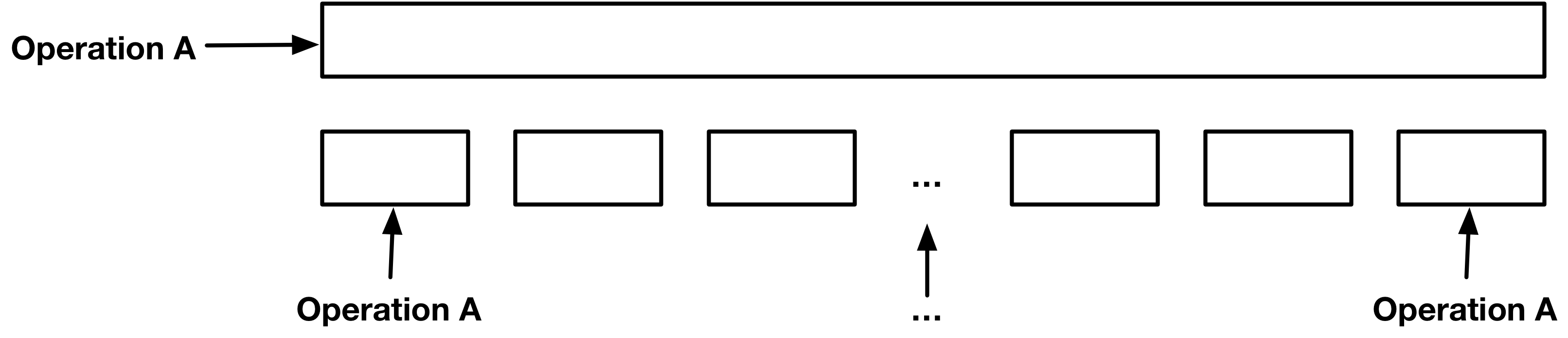
Data parallelism is, given a dataset, the simultaneous execution on multiple machines or threads of the same function across groups of elements of a dataset. Data parallelism can also be thought of as a subset of SIMD (“single instruction, multiple data”) execution, a class of parallel execution in Flynn’s taxonomy. Comparably, one could think a sequential computation as “for all elements in the dataset, do operation A” on a single big dataset, whose size can reach to terabytes or petabytes. The challenges to doing this sequential computation in a parallelized manner include how to abstract the different types of computations in a simple and correct way, how to distribute the data to hundreds/thousands of machines or clusters, and how to schedule tasks and handle failures.

MapReduce (Dean & Ghemawat, 2008) is a programming model proposed by Google to initially satisfy their demand of large-scale indexing for web search service. It provides a simple user program interface: map and reduce functions and automatically handles the parallelization and distribution. The underlying execution systems can provide fault tolerance and scheduling.

The MapReduce model is simple and powerful and quickly becomes very popular among developers. However, when developers start writing real-world applications, they often end up writing many pieces of boilerplate code and chaining together these stages. Moreover, The pipeline of MapReduce forces them to write additional coordinating codes, i.e., the development style goes backward from simple logic computation abstraction to lower-level coordination management. As we will discuss in section 2 execution model, MapReduce writes all data into disk after each stage, which causes severe delays. Programmers need to do manual optimizations for targeted performance, and this again requires them to understand the underlying execution model. The whole process soon becomes cumbersome. The FlumeJava (Chambers et al., 2010) library intends to provide support for developing data-parallel pipelines by abstracting away the complexity involved in data representation and implicitly handling the optimizations. It defers the evaluation, constructs an execution plan from parallel collections, optimizes the plan, and then executes underlying MR primitives. The optimized execution is comparable with hand-optimized pipelines, thus there is no much need to write raw MR programs directly.

After MapReduce, Microsoft proposed their counterpart data parallelism model, Dryad (Isard, Budiu, Yu, Birrell, & Fetterly, 2007), which abstracts individual computational tasks as vertices, and constructs a communication graph between those vertices. What programmers need to do is to describe this DAG and let the Dryad execution engine construct the execution plan and manage scheduling and optimization. One of the advantages of Dryad over MapReduce is that Dryad vertices can process an arbitrary number of inputs and outputs, while MR only supports a single input and a single output for each vertex. Besides the flexibility of computations, Dryad also supports different types of communication channel: file, TCP pipe, and shared-memory FIFO. The programming model is less elegant than MapReduce, as programmers are not meant to interact with it directly. Instead, they are expected to use the high-level programming interface DryadLinq (Yu et al., 2008), which is more expressive and better embedded within the .NET framework. We can see some examples later in the section devote to Dryad.

Dryad expresses computation as acyclic data flows, which might be too expensive for some complex applications e.g. iterative machine learning algorithms. Spark (Zaharia, Chowdhury, Franklin, Shenker, & Stoica, 2010) is a framework that uses functional programming and pipelining to provide such support. Spark is largely inspired by MapReduce’s model and builds upon the ideas behind using DAGs and lazy evaluation found in DryadLinq. Instead of writing data to disk for each job as MapReduce does Spark can cache the results across jobs. Spark explicitly caches computational data in memory through specialized immutable data structure named Resilient Distributed Sets (RDD) and reuse the same dataset across multiple parallel operations. The Spark builds upon RDDs to achieve fault tolerance by reusing the lineage information of the lost RDD. This results in less overhead than what is seen in fault tolerance achieved by using checkpoints in Distributed Shared Memory systems. Moreover, Spark is the underlying framework upon which many very different systems are built e.g. Spark SQL & DataFrames, GraphX, Streaming Spark, which makes it easy to mix and match the use of these systems all in the same application. These features make Spark the best fit for iterative jobs and interactive analytics and also help it to provide better performance.

The following four sections discuss the programming models of MapReduce, FlumeJava, Dryad, and Spark.

MapReduce

In this model, parallelizable computations are abstracted into map and reduce functions. The computation accepts a set of key/value pairs as input and produces a set of key/value pairs as output. The process involves two phases:

• Map, written by the user, accepts a set of key/value pairs (a “record”) as input, applies map operation on each record, and computes a set of intermediate key/value pairs as output.
• Reduce, also written by the user, accepts an intermediate key and a set of values associated with that key, operates on them, and produces zero or one output value.

Note: there is also a Shuffle phase between Map and Reduce, provided by MapReduce library, which groups all the intermediate values of the same key together and passes them to the Reduce function. This is discussed more in the section on Execution Models.

Conceptually, the map and reduce functions have associated types:

\[map (k1,v1) \rightarrow list(k2,v2)\]

\[reduce (k2,list(v2)) \rightarrow list(v2)\]

The input keys and values are drawn from a different domain than the output keys and values. The intermediate keys and values are from the same domain as the output keys and values.

As an example, we can consider the problem of counting the number of occurrences of each word in a large collection of documents. This could be modeled as a map function that emits a word plus its count 1 and a reduce function which sums together all the counts emitted for the same word. Pseudocode of the map and reduce phases to solve this problem is given below.

map(String key, String value):
  // key: document name
  // value: document contents
  for each word in value:
    EmitIntermediate(word, "1");

reduce(String key, Iterator values):
  // key: a word
  // values: a list of counts
  int result = 0;
  for each value in values:
    result += ParseInt(value);
  Emit(AsString(result));

During execution, the MapReduce library assigns a master node to manage data partition and scheduling. Other nodes can serve as workers to run either map or reduce operations on demand. More details of the execution model are discussed later. Here, it’s worth mentioning that the intermediate results output by the map phase are written to disk and the reduce operation then reads its input from disk. This is crucial for fault tolerance.

Fault Tolerance

MapReduce runs on hundreds or thousands of unreliable commodity machines, so the library must provide fault tolerance. The library assumes that master node will not fail, and it monitors worker failures. If no status update is received from a worker on timeout, the master will mark it as failed. Then the master may schedule the associated task to other workers depending on task type and status. The commits of map and reduce task outputs are atomic, where the in-progress task writes data into private temporary files, and then once the task succeeds, it negotiates with the master and renames files to complete the task. In the case of failure, the worker discards those temporary files. This guarantees that if the computation is deterministic, the distributed implementation should produce the same outputs as a failure-free sequential execution.

Limitations

Many analytics workloads like K-means, logistic regression, graph processing applications like PageRank, and shortest path using parallel breadth-first search require multiple stages of MapReduce jobs. In a regular MapReduce framework like Hadoop, this requires the developer to manually handle the iterations in the driver code. At every iteration, the result of each stage T is written to HDFS and loaded back again at stage T+1 causing a performance bottleneck. The reason for this is waste of network bandwidth, CPU resources, and primarily inherently slow disk I/O operations. In order to address such challenges in iterative workloads on MapReduce, frameworks like Haloop (Bu, Howe, Balazinska, & Ernst, 2010), Twister (Ekanayake et al., 2010), and iMapReduce (Zhang, Gao, Gao, & Wang, 2012) adopt special techniques like caching the data between iterations and keeping the mapper and reducer alive across the iterations.

FlumeJava

FlumeJava (Chambers et al., 2010) was introduced to make it easy to develop, test, and run efficient data-parallel pipelines. FlumeJava represents each dataset as an object and transformation is invoked by applying methods on these objects. It constructs an efficient internal execution plan from a pipeline of MapReduce jobs, uses deferred evaluation and optimizes based on plan structures. The debugging ability allows programmers to run on their local machine first and then deploy their job to large clusters.

Core Abstractions

• PCollection<T>, a immutable bag of elements of type T, which can be created from an in-memory Java Collection<T> or from reading a file with encoding specified by recordOf.
• recordOf(...), specifies the encoding of the instance
• PTable<K, V>, a subclass of PCollection<Pair<K,V>>, an immutable multi-map with keys of type K and values of type V
• parallelDo(), can express both the map and reduce parts of MapReduce
• groupByKey(), same as shuffle step of MapReduce
• combineValues(), semantically a special case of parallelDo(), a combination of a MapReduce combiner and a MapReduce reducer, which is more efficient than doing all the combining in the reducer.
• flatten, takes a list of PCollection<T>s and returns a single PCollection<T>.

An example implemented using FlumeJava:

PTable<String, Integer> wordsWithOnes =
  words.parallelDo(
    new DoFn<String, Pair<String, Integer>> () {
      void process(String word,
                   EmitFn<Pair<String, Integer>> emitFn) {
        emitFn.emit(Pair.of(word, 1));
      }
    }, tableOf(strings(), ints()));
PTable<String, Collection<Integer>>
  groupedWordsWithOnes = wordsWithOnes.groupByKey();
PTable<String, Integer> wordCounts =
  groupedWordsWithOnes.combineValues(SUM_INTS);

Deferred Evaluation & Optimization

One of the merits of using FlumeJava to pipeline MapReduce jobs is that it enables optimization automatically, by executing parallel operations lazily using deferred evaluation. The state of each PCollection object is either deferred (not yet computed) and materialized (computed). When the program invokes a parallelDo(), it creates an operation pointer to the actual deferred operation object. These operations form a directed acyclic graph called execution plan. The execution plan doesn’t get evaluated until run() is called. This will cause optimization of the execution plan and evaluation in forward topological order. These optimization strategies for transferring the modular execution plan into an efficient one include:

• Fusion: $f(g(x)) => g \circ f(x)$, which is essentially function composition. This usually help reduce the number of steps need for a given job by combining multiple composable steps into one.
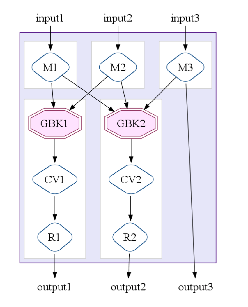
• MapShuffleCombineReduce (MSCR) Operation: a combination of ParallelDo, GroupByKey, CombineValues and Flatten into one MapReduce job. This extends MapReduce to accept multiple inputs and multiple outputs. Following figure illustrates the case a MSCR operation with 3 input channels, 2 grouping (GroupByKey) output channels and 1 pass-through output channel.

An overall optimizer strategy involves a sequence of optimization actions with the ultimate goal to produce the fewest, most efficient MSCR operations:

1. Sink Flatten: $h(f(a)+g(b)) \rightarrow h(f(a)) + h(g(b))$
2. Lift combineValues operations: If a CombineValues operation immediately follows a GroupByKey operation, the GroupByKey records the fact and original CombineValues is left in place, which can be treated as normal ParallelDo operation and subject to ParallelDo fusions.
3. Insert fusion blocks:
4. Fuse ParallelDos
5. Fuse MSCRs: create MSCR operations, and convert any remaining unfused ParallelDo operations into trivial MSCRs.

The SiteData example (Chambers et al., 2010) shows that 16 data-parallel operations can be optimized into two MSCR operations in the final execution plan (refer to Figure 5 in the original paper). One limitation of the optimizer is that all these optimizations are based on the structures of the execution plan, FlumeJava doesn’t analyze the contents of user-defined functions.

Dryad

Dryad is a general-purpose data-parallel execution engine that allows developers to explicitly specify an arbitrary directed acyclic graph (DAG) for computations, where each vertex is a computation task and the edges represent communication channels (file, TCP pipe, or shared-memory FIFI) between tasks.

A Dryad job is a logic computation graph that is automatically mapped to physical resources at runtime. From a programmer’s point of view, the channels produce or consume heap objects and the type of data channel makes no difference when reading or writing these objects. In the Dryad system, a process called a “job manager” connects to the cluster network and is responsible for scheduling jobs by consulting the name server (NS) and delegating commands to the daemon (D) running on each computer in the cluster.

Writing a program

The Dryad library is written in C++ and it uses a mixture of method calls and operator overloading. It describes a Dryad graph as $G=\langle V_G, E_G, I_G, O_G \rangle$, where $V_G$ is a sequences of vertices, $E_G$ is a set of directed edges, $I_G$ and $O_G$ represent vertices for inputs and outputs.

• Creating new vertices The library calls static program factory to create a graph vertex and it also provides $^$ operator to clone a graph and $\otimes$ to concatenate sequences.
• Adding graph edges $C=A\circ B$ creates a new graph $C=\langle V_A \otimes V_B, E_A \cup E_B \cup E_{new}, I_A, O_B \rangle$. The composition of set of edges are defined by two types:
  1) $A>=B$ pointwise composition
  2) and $A>>B$ complete bipartite graph between $O_A$ and $I_B$.
• Merging two graphs $C=A \mid\mid B$ creates a new graph $C=\langle V_A \otimes^* V_B, E_A \cup E_B, I_A \cup^* I_B, O_A\cup^* O_B \rangle$.

Following is an example graph builder program.

GraphBuilder XSet = moduleX^N;
GraphBuilder DSet = moduleD^N;
GraphBuilder MSet = moduleM^(N*4);  
GraphBuilder SSet = moduleS^(N*4);
GraphBuilder YSet = moduleY^N;
GraphBuilder HSet = moduleH^1;

GraphBuilder XInputs = (ugriz1 >= XSet) || (neighbor >= XSet);
GraphBuilder YInputs = ugriz2 >= YSet;

GraphBuilder XToY = XSet >= DSet >> MSet >= SSet;

for (i = 0; i < N*4; ++i)
{
  XToY = XToY || (SSet.GetVertex(i) >= YSet.GetVertex(i/4));
}
GraphBuilder YToH = YSet >= HSet;
GraphBuilder HOutputs = HSet >= output;

GraphBuilder final = XInputs || YInputs || XToY || YToH || HOutputs;

Developers are not expected to write raw Dryad programs as complex as the one shown above. Instead, Microsoft introduced a querying model called DryadLINQ (Yu et al., 2008) which is more declarative. We will discuss querying models and their power to express complex operations like join in section 1.2 Querying. Here we just show a glimpse of querying example in DryadLINQ (who is compiled into Dryad jobs and executed in Dryad execution engine):

// SQL-style syntax to join two input sets:
// scoreTriples and staticRank
var adjustedScoreTriples =
  from d in scoreTriples
  join r in staticRank on d.docID equals r.key
  select new QueryScoreDocIDTriple(d, r);
var rankedQueries =
  from s in adjustedScoreTriples
  group s by s.query into g
  select TakeTopQueryResults(g);

// Object-oriented syntax for the above join
var adjustedScoreTriples =
  scoreTriples.Join(staticRank,
    d => d.docID, r => r.key,
    (d, r) => new QueryScoreDocIDTriple(d, r));
var groupedQueries =
  adjustedScoreTriples.GroupBy(s => s.query);
var rankedQueries =
  groupedQueries.Select(
    g => TakeTopQueryResults(g));

Fault tolerance policy

The communication graph is acyclic, so if given immutable inputs, the computation result should remain same regardless of the sequence of failures. When a vertex fails, the job manager will either get notified or receive a heartbeat timeout and then the job manager will immediately schedule to re-execute the vertex.

Comparison with FlumeJava

Both support multiple inputs/outputs for the computation nodes. The big difference is that FlumeJava still exploits the MapReduce approach to reading from/writing to disks between stages, where Dryad has the option to do in-memory transmission. This leaves Dryad a good position to do optimization like re-using in-memory data. In the other hand, Dryad has no optimizations on the graph itself.

Spark

Spark (Zaharia, Chowdhury, Franklin, Shenker, & Stoica, 2010) is a fast, in-memory data processing engine with an elegant and expressive development interface which enables developers to efficiently execute machine learning, SQL or streaming workloads that require fast iterative access to datasets. It is a functional style programming model (similar to DryadLINQ) where a developer can create acyclic data flow graphs and transform a set of input data through a map - reduce like operators. Spark provides two main abstractions: distributed in-memory storage (RDD) and parallel operations (based on Scala’s collection API) on data sets with high-performance processing, scalability, and fault tolerance. 

Distributed in-memory storage - Resilient Distributed Data sets

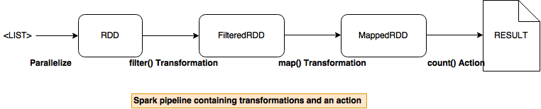
A RDD is a partitioned, read-only collection of objects which can be created from data in stable storage or by transforming other RDD. It can be distributed across multiple nodes (parallelize) in a cluster and is fault tolerant(resilient). If a node fails, an RDD can always be recovered using its lineage; the DAG of computations performed on the source dataset. An RDD is stored in memory (as much as it can fit and rest is spilled to disk) and is immutable - It can only be transformed to a new RDD. These transformations are deferred; that means they are built up and staged and are not actually applied until an action is performed on an RDD. Thus, it is important to note that while one might have applied many transformations to a given RDD, some resulting transformed RDD may not be materialized even though one may hold a reference to it.

The properties that power RDD with the above-mentioned features:

• A list of dependencies on other RDD’s.
• An array of partitions that a dataset is divided into.
• A compute function to do a computation on partitions.
• Optionally, a Partitioner for key-value RDDs (e.g. to say that the RDD is hash-partitioned)
• Optional preferred locations (aka locality info), (e.g. block locations for an HDFS file)

Spark API provide two kinds of operations on an RDD:

• Transformations - lazy operations that return another RDD.
  • map (f : T => U) : RDD[T] ⇒ RDD[U] Return a MappedRDD[U] by applying function f to each element
  • flatMap( f : T ⇒ Seq[U]) : RDD[T] ⇒ RDD[U] Return a new FlatMappedRDD[U] by first applying a function to all elements  and then flattening the results.
  • filter(f:T⇒Bool) : RDD[T] ⇒ RDD[T] Return a FilteredRDD[T] having elemnts that f return true
  • groupByKey() Being called on (K,V) Rdd, return a new RDD[([K], Iterable[V])]
  • reduceByKey(f: (V, V) => V) : Being called on (K, V) Rdd, return a new RDD[(K, V)] by aggregating values using eg: reduceByKey(+)
  • join((RDD[(K, V)], RDD[(K, W)]) ⇒ RDD[(K, (V, W))] Being called on (K,V) Rdd, return a new RDD[(K, (V, W))] by joining them by key K.

• Actions - operations that trigger computation on an RDD and return values.

  • reduce(f:(T,T)⇒T) : RDD[T] ⇒ T Return T by reducing the elements using specified commutative and associative binary operator
  • collect() Return an Array[T] containing all elements
  • count() Return the number of elements

RDDs by default are discarded after use. However, Spark provides two explicit operations: persist() and cache() to ensure RDDs are persisted in memory once the RDD has been computed for the first time.

Why RDD, not Distributed Shared memory (DSM) ?

RDDs are immutable and can only be created through coarse-grained transformations while DSM allows fine-grained read and write operations to each memory location. Since RDDs are immutable and can be derived from their lineages, they do not require checkpointing at all. Hence RDDs do not incur the overhead of checkpointing as DSM does. Additionally, in DSM, any failure requires the whole program to be restored. In the case of RDDs, only the lost RDD partitions need to be recovered. This recovery happens parallelly on the affected nodes. RDDs are immutable and hence a straggler (slow node) can be replaced with a backup copy as in MapReduce. This is hard to implement in DSM as two copies point to the same location and can interfere the update with one another.

Challenges in Spark (Armbrust et al., 2015)

• Functional API semantics The GroupByKey operator is costly in terms of performance. In that it returns a distributed collection of (key, list of value) pairs to a single machine and then an aggregation on individual keys is performed on the same machine resulting in computation overhead. Spark does provide reduceByKey operator which does a partial aggregation on individual worker nodes before returning the distributed collection. However, developers who are not aware of such a functionality can unintentionally choose groupByKey. The reason being functional programmers (Scala developers) tend to think more declaratively about the problem and only see the end result of the groupByKey operator. They may not be necessarily trained on how groupByKey is implemented atop of the cluster. Therefore, to use Spark, unlike functional programming languages, one needs to understand how the underlying cluster is going to execute the code. The burden of saving performance is then left to the programmer, who is expected to understand the underlying execution model of Spark, and to know when to use reduceByKey over groupByKey.

• Debugging and profiling There is no availability of debugging tools and developers find it hard to realize if a computation is happening more on a single machine or if the data-structure they used were inefficient.

Querying: declarative interfaces

MapReduce takes care of all the processing over a cluster, failure and recovery, data partitioning etc. However, the framework suffers from rigidity with respect to its one-input data format (key/value pair) and two-stage data flow. Several important patterns like equi-joins and theta-joins (Okcan & Riedewald, 2011) which could be highly complex depending on the data, require programmers to implement by hand. Hence, MapReduce lacks many such high level abstractions requiring programmers to be well versed with several of the design patterns like map-side joins, reduce-side equi-join etc. Also, java based code (like in Hadoop framework) in MapReduce can sometimes become repetitive when the programmer wants to implement most common operations like projection, filtering etc. A simple word count program as shown below, can span up to 63 lines.

Complete code for Word count in Hadoop (Java based implementation of MapReduce)

import java.io.IOException;
import java.util.*;
import org.apache.hadoop.fs.Path;
import org.apache.hadoop.conf.*;
import org.apache.hadoop.io.*;
import org.apache.hadoop.mapreduce.*;
import org.apache.hadoop.mapreduce.lib.input.FileInputFormat;
import org.apache.hadoop.mapreduce.lib.input.TextInputFormat;
import org.apache.hadoop.mapreduce.lib.output.FileOutputFormat;
import org.apache.hadoop.mapreduce.lib.output.TextOutputFormat;

public class WordCount
{
   public static class Map extends Mapper<LongWritable, Text, Text,  IntWritable>
   {
    private final static IntWritable one = new IntWritable(1);
    private Text word = new Text();

    public void map(LongWritable key, Text value, Context context) throws IOException, InterruptedException
    {
     String line = value.toString();
     StringTokenizer tokenizer = new StringTokenizer(line);
     while (tokenizer.hasMoreTokens())
     {
        word.set(tokenizer.nextToken());
        context.write(word, one);
     }
  }

  public static class Reduce extends Reducer<Text, IntWritable, Text, IntWritable>
  {
   public void reduce(Text key, Iterable<IntWritable> values, Context context) throws IOException, InterruptedException
   {
     int sum = 0;
     for (IntWritable val : values)
     {
       sum += val.get();
     }
     context.write(key, new IntWritable(sum));
   }
  }

  public static void main(String[] args) throws Exception
  {
    Configuration conf = new Configuration();
    Job job = new Job(conf, "wordcount");
    job.setOutputKeyClass(Text.class);
    job.setOutputValueClass(IntWritable.class);
    job.setMapperClass(Map.class);
    job.setReducerClass(Reduce.class);
    job.setInputFormatClass(TextInputFormat.class);
    job.setOutputFormatClass(TextOutputFormat.class);
    FileInputFormat.addInputPath(job, new Path(args[0]));
    FileOutputFormat.setOutputPath(job, new Path(args[1]));
  }

  job.waitForCompletion(true);
}

Why SQL over MapReduce ?

SQL already provides several operations like join, group by, sort which can be mapped to the above mentioned MapReduce operations. Also, by leveraging SQL like interface, it becomes easy for non MapReduce experts/non-programmers like data scientists to focus more on logic than hand coding complex operations (Armbrust et al., 2015). Such an high level declarative language can easily express their task while leaving all of the execution optimization details to the backend engine.

SQL also lessens the amount of code (code examples can be seen in individual model’s section) and significantly reduces the development time.

Most importantly, as you will read further in this section, frameworks like Pig, Hive, Spark SQL take advantage of these declarative queries by realizing them as a DAG upon which the compiler can apply transformation if an optimization rule is satisfied. Spark which does provide high level abstraction unlike MapReduce, lacks this very optimization resulting in several human errors as discussed in the Spark’s data-parallel section.

Sawzall (Pike, Dorward, Griesemer, & Quinlan, 2005) is a programming language built on top of MapReduce. It consists of a filter phase (map) and an aggregation phase (reduce). User program only need to specify the filter function, and emit the intermediate pairs to external pre-built aggregators. This largely eliminates the trouble for programmers put into having to write reducers, just the following example shows, programmers can use built-in reducer supports to do the a reducing job. The serialization of the data uses Google’s protocol buffers, which can produce meta-data file for the declared scheme, but the scheme is not used for any optimization purpose per se. Sawzall is good for most of the straightforward processing on large dataset, but it does not support more complex and still common operations like join. The pre-built aggregators are limited and it is non-trivial to add more supports.

• Word count implementation in Sawzall

result: table sum of int;
total: table sum of float;
x: float = input;
emit count <- 1;
emit total <- x;

Apart from Sawzall, Pig (Olston, Reed, Srivastava, Kumar, & Tomkins, 2008) and Hive (Thusoo et al., 2009) are the other major components that sit on top of Hadoop framework for processing large data sets without the users having to write Java based MapReduce code. Both support more complex operations than Sawzall: e.g. database join.

Hive is built by Facebook to organize dataset in structured formats and still utilize the benefit of MapReduce framework. It has its own SQL-like language: HiveQL (Thusoo et al., 2010) which is easy for anyone who understands SQL. Hive reduces code complexity and eliminates lots of boiler plate that would otherwise be an overhead with Java based MapReduce approach.

• Word count implementation in Hive

CREATE TABLE docs (line STRING);
LOAD DATA INPATH 'docs' OVERWRITE INTO TABLE docs;
CREATE TABLE word_counts AS
SELECT word, count(1) AS count FROM
(SELECT explode(split(line, '\\s')) AS word FROM docs) w
GROUP BY word
ORDER BY word;

Pig Latin by Yahoo aims at a sweet spot between declarative and procedural programming. For advanced programmers, SQL is unnatural to implement program logic and Pig Latin wants to dissemble the set of data transformation into a sequence of steps. This makes Pig more verbose than Hive. Unlike Hive, Pig Latin does not persist metadata, instead it has better interoperability to work with other applications in Yahoo’s data ecosystem.

• Word count implementation in PIG

lines = LOAD 'input_fule.txt' AS (line:chararray);
words = FOREACH lines GENERATE FLATTEN(TOKENIZE(line)) as word;
grouped = GROUP words BY word;
wordcount = FOREACH grouped GENERATE group, COUNT(words);
DUMP wordcount;

SparkSQL though has the same goals as that of Pig, is better given the Spark exeuction engine, efficient fault tolerance mechanism of Spark and specialized data structure called Dataset.

• Word count example in SparkSQL

val ds = sqlContext.read.text("input_file").as[String]
val result = ds
  .flatMap(_.split(" "))              
  .filter(_ != "")                    
  .toDF()                             
  .groupBy($"value")                 
  .agg(count("*") as "count")
  .orderBy($"count" desc)   

The following subsections will discuss Hive, Pig Latin, SparkSQL in details.

Hive/HiveQL

Hive (Thusoo et al., 2010) is a data-warehousing infrastructure built on top of the MapReduce framework - Hadoop. The primary responsibility of Hive is to provide data summarization, query, and analysis. It supports analysis of large datasets stored in Hadoop’s HDFS (Shvachko, Kuang, Radia, & Chansler, 2010). It supports SQL-Like access to structured data which is known as HiveQL (or HQL) as well as big data analysis with the help of MapReduce. These SQL queries can be compiled into MapReduce jobs that can be executed be executed on Hadoop. It drastically brings down the development time in writing and maintaining Hadoop jobs.

Data in Hive is organized into three different formats:

Tables: Like RDBMS tables Hive contains rows and tables and every table can be mapped to HDFS directory. All the data in the table is serialized and stored in files under the corresponding directory. Hive is extensible to accept user-defined data formats, customized serialize and de-serialize methods. It also supports external tables stored in other native file systems like HDFS, NFS or local directories.

Paritions: Distribution of data in sub directories of table directory is determined by one or more partitions. A table can be further partitioned on columns.

Buckets: Data in each partition can be further divided into buckets on the basis on hash of a column in a table. Each bucket is stored as a file in the partition directory.

HiveSQL: The Hive query language consists of a subset of SQL along with some extensions. The language is very SQL-like and supports features like subqueries, joins, cartesian product, group by, aggregation, describe and more. MapReduce programs can also be used in Hive queries. A sample query using MapReduce would look like this:

FROM (
    MAP inputdata USING 'python mapper.py' AS (word, count)
    FROM inputtable
    CLUSTER BY word
    )
    REDUCE word, count USING 'python reduce.py';

Example from (Thusoo et al., 2010)

This query uses mapper.py for transforming inputdata into (word, count) pair, distributes data to reducers by hashing on word column (given by CLUSTER) and uses reduce.py.

Serialization/Deserialization

Hive implements the LazySerDe as the default SerDe interface. A SerDe is a combination of serialization and deserialization which helps developers instruct Hive on how their records should be processed. The Deserializer interface translates rows into internal objects lazily so that the cost of Deserialization of a column is incurred only when it is needed. The Serializer, however, converts a Java object into a format that Hive can write to HDFS or another supported system. Hive also provides a RegexSerDe which allows the use of regular expressions to parse columns out from a row.

Pig Latin

Pig Latin (Olston, Reed, Srivastava, Kumar, & Tomkins, 2008) is a programming model built on top of MapReduce to provide a declarative description. Different from Hive, who has SQL-like syntax, the goal of Pig Latin is to attract experienced programmers to perform ad-hoc analysis on big data and allow programmers to write execution logic by a sequence of steps. For example, suppose we have a table URLs: (url, category, pagerank). The following is a simple SQL query that finds, for each sufficiently large category, the average pagerank of high-pagerank URLs in that category.

SELECT category, AVG(pagerank)  
FROM urls WHERE pagerank > 0.2  
GROUP BY category HAVING COUNT(*) > 106  

And Pig Latin provides an alternative to carrying out the same operations in the way programmers can reason more easily:

good_urls = FILTER urls BY pagerank > 0.2;
groups = GROUP good_urls BY category;
big_groups = FILTER groups BY COUNT(good_urls)>106;
output = FOREACH big_groups GENERATE
            category, AVG(good_urls.pagerank);

Interoperability Pig Latin is designed to support ad-hoc data analysis, which means the input only requires a function to parse the content of files into tuples. This saves the time-consuming import step. While as for the output, Pig provides freedom to convert tuples into byte sequence where the format can be defined by users. This allows Pig to interoperate with other existing applications in Yahoo’s ecosystem.

Nested Data Model Pig Latin has a flexible, fully nested data model, and allows complex, non-atomic data types such as set, map, and tuple to occur as fields of a table. The benefits include: closer to how programmer think; data can be stored in the same nested fashion to save recombining time; can have algebraic language; allow rich user defined functions.

UDFs as First-Class Citizens Pig Latin supports user-defined functions (UDFs) to support customized tasks for grouping, filtering, or per-tuple processing, which makes Pig Latin more declarative.

Debugging Environment Pig Latin has a novel interactive debugging environment that can generate a concise example data table to illustrate the output of each step.

Limitations The procedural design gives users more control over execution, but at same time the data schema is not enforced explicitly, so it much harder to utilize database-style optimization. Pig Latin has no control structures like loop or conditions, if needed, one has to embed it in Java like JDBC style, but this can easily fail without static syntax checking. It is also not easy to debug.

SparkSQL

The major contributions of Spark SQL (Armbrust et al., 2015) are the Dataframe API and the Catalyst. Spark SQL intends to provide relational processing over native RDDs and on several external data sources, through a programmer friendly API, high performance through DBMS techniques, support semi-structured data and external databases, support for advanced analytical processing like machine learning algorithms and graph processing.

Programming API

Spark SQL runs on the top of Spark providing SQL interfaces. A user can interact with this interface through JDBC/ODBC, command line or Dataframe API.

The Dataframe API lets users to intermix both relational and procedural code with ease. Dataframe is a collection of schema based rows of data and named columns on which relational operations can be performed with optimized execution. Unlike an RDD, Dataframe allows developers to define the structure for the data and can be related to tables in a relational database or R/Python’s Dataframe. Dataframe can be constructed from tables of external sources or existing native RDD’s. Dataframe is lazy and each object in it represents a logical plan which is not executed until an output operation like save or count is performed. Spark SQL supports all the major SQL data types including complex data types like arrays, maps, and unions. Some of the Dataframe operations include projection (select), filter(where), join and aggregations(groupBy).

Illustrated below is an example of relational operations on employees data frame to compute the number of female employees in each department.

employees.join(dept, employees("deptId") === dept("id"))
         .where(employees("gender") === "female")
         .groupBy(dept("id"), dept("name"))
         .agg(count("name"))

Several of these operators like === for equality test, > for greater than, arithmetic ones (+, -, etc) and aggregators transforms to an abstract syntax tree of the expression which can be passed to Catalyst for optimization.

A cache() operation on the data frame helps Spark SQL store the data in memory so it can be used in iterative algorithms and for interactive queries. In the case of Spark SQL, memory footprint is considerably less as it applies columnar compression schemes like dictionary encoding / run-length encoding.

The DataFrame API also supports inline UDF definitions without complicated packaging and registration. Because UDFs and queries are both expressed in the same general purpose language (Python or Scala), users can use standard debugging tools.

However, a DataFrame lacks type safety. In the above example, attributes are referred to by string names. Hence, it is not possible for the compiler to catch any errors. If attribute names are incorrect then the error will only be detected at runtime, when the query plan is created.

Also, Dataframe is both very brittle and very verbose as well, because the user has to cast each row and column to specific types before they can do anything on them. Naturally, this is very error-prone because one could accidentally choose the wrong index for a row/column and end up with a ClassCastException.

Spark introduced an extension to Dataframe called Dataset to provide this compile type safety. It embraces object-oriented style for programming and has an additional feature termed Encoders. Encoders translate between JVM representations (objects) and Spark’s internal binary format. Spark has built-in encoders which are very advanced in that they generate bytecode to interact with off-heap data and provide on-demand access to individual attributes without having to de-serialize an entire object

Winding up - we can compare SQL vs Dataframe vs Dataset as below:

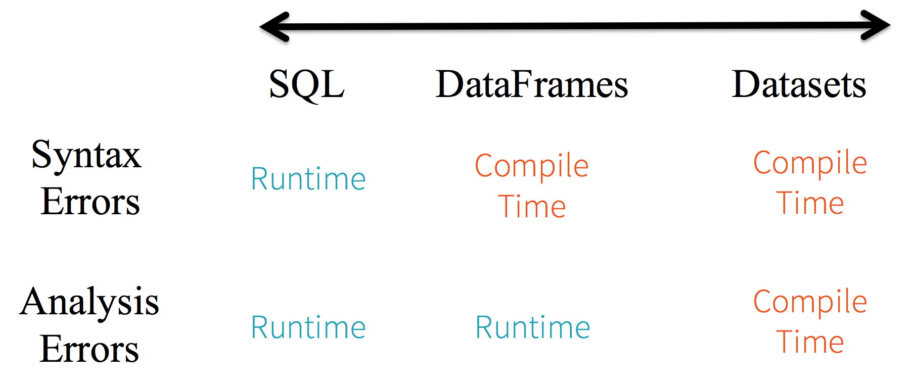
Figure from the website : https://databricks.com/blog/2016/07/14/a-tale-of-three-apache-spark-apis-rdds-dataframes-and-datasets.html

Large-scale parallelism on graphs

MapReduce doesn’t scale easily for iterative / graph algorithms like page rank and machine learning algorithms. Iterative algorithms require a programmer to explicitly handle the intermediate results (writing to disks) resulting in a lot of boilerplate code. Hence, every iteration requires reading the input file and writing the results to the disk resulting in high disk I/O which is a performance bottleneck for any batch processing system.

Also, graph algorithms require an exchange of messages between vertices. In a case of PageRank, every vertex requires the contributions from all its adjacent nodes to calculate its score. MapReduce currently lacks this model of message passing which makes it complex to reason about graph algorithms. One model that is commonly employed for implementing distributed graph processing is the graph parallel model.

In the graph-parallel abstraction, a user-defined vertex program is instantiated concurrently for each vertex and interacts with adjacent vertex programs through messages or shared state. Each vertex program can read and modify its vertex property and in some cases adjacent vertex properties. When all vertex programs vote to halt the program terminates. The bulk-synchronous parallel (BSP) model (Valiant, 1990) is one of the most commonly used graph-parallel model.

BSP was introduced in 1980 to represent the hardware design features of parallel computers. It gained popularity as an alternative for MapReduce since it addressed the above-mentioned issues with MapReduce BSP model is a message passing synchronous model where -

• Computation consists of several steps called as super steps.
• The processors involved have their own local memory and every processor is connected to other via a point-to-point communication.
• At every super step, a processor receives input at the beginning, performs computation and outputs at the end.
• A processor at super step S can send a message to another processor at super step S+1 and can as well receive a message from super step S-1.
• Barrier synchronization syncs all the processors at the end of every super step.
• A notable feature of the model is the complete control of data through communication between every processor at every super step. Though similar to MapReduce model, BSP preserves data in memory across super steps and helps in reasoning iterative graph algorithms.

The graph-parallel abstractions allow users to succinctly describe graph algorithms, and provide a runtime engine to execute these algorithms in a distributed nature. They simplify the design, implementation, and application of sophisticated graph algorithms to large-scale real-world problems. Each of these frameworks presents a different view of graph computation, tailored to an originating domain or family of graph algorithms. However, these frameworks fail to address the problems of data preprocessing and construction, favor snapshot recovery over fault tolerance and lack support from distributed data flow frameworks. The data-parallel systems are well suited to the task of graph construction and are highly scalable. However, suffer from the very problems mentioned before for which the graph-parallel systems came into existence. GraphX (Xin, Gonzalez, Franklin, & Stoica, 2013) is a new computation system which builds upon the Spark’s Resilient Distributed Dataset (RDD) to form a new abstraction Resilient Distributed Graph (RDG) to represent records and their relations as vertices and edges respectively. RDG’s leverage the RDD’s fault tolerance mechanism and expressivity.

How does GraphX improve over the existing graph-parallel and data flow models?

Similar to the data flow model, GraphX moves away from the vertex-centric view and adopts transformations on graphs yielding a new graph. The RDGs in GraphX provides a set of elegant and expressive computational primitives to support graph transformations as well as enable many graph-parallel systems like Pregel (Malewicz et al., 2010), PowerGraph (Gonzalez, Low, Gu, Bickson, & Guestrin, 2012) to be easily expressed with minimal lines of code changes to Spark. GraphX simplifies the process of graph ETL and analysis through new operations like filter, view etc. It minimizes communication and storage overhead across the system by adopting vertex-cuts for effective partitioning.

GraphX

GraphX models graph as property graphs where vertices and edges can have properties. Property graphs are directed multigraph having multiple parallel edges with same source and destination to realize scenarios where multiple relationships could exist between two vertices. For example, in a social graph where every vertex represents a person, there could be a scenario where two people are both co-workers and a friend at the same time. A vertex is keyed by a unique 64-bit long identifier (Vertex ID) while edges contain the corresponding source and destination vertex identifiers.

The GraphX API provides the below primitives for graph transformations (from: https://spark.apache.org/docs/2.0.0-preview/graphx-programming-guide.html):

• graph - constructs property graph given a collection of edges and vertices.
• vertices: VertexRDD[VD], edges: EdgeRDD[ED]- decompose the graph into a collection of vertices or edges by extracting vertex or edge RDDs.
• mapVertices(map: (Id,V)=>(Id,V2)) => Graph[V2, E]- transform the vertex collection.
• mapEdges(map: (Id, Id, E)=>(Id, Id, E2)) - transform the edge collection.
• triplets RDD[EdgeTriplet[VD, ED]] -returns collection of form ((i, j), (PV(i), PE(i, j), PV(j))). The operator essentially requires a multiway join between vertex and edge RDD. This operation is optimized by shifting the site of joins to edges, using the routing table, so that only vertex data needs to be shuffled.
• leftJoin - given a collection of vertices and a graph, returns a new graph which incorporates the property of matching vertices from the given collection into the given graph without changing the underlying graph structure.
• subgraph - Applies predicates to return a subgraph of the original graph by filtering all the vertices and edges that don’t satisfy the vertices and edges predicates respectively.
• aggregateMessages (previously mapReduceTriplets) - It takes two functions, sendMsg and mergeMsg. The sendMsg function maps over every edge triplet in the graph while the mergeMsg acts like a reduce function in MapReduce to aggregate those messages at their destination vertex. This is an important function which supports analytics tasks and iterative graph algorithms (eg., PageRank, Shortest Path) where individual vertices rely upon the aggregated properties of their neighbors.
• filterVertices(f: (Id, V)=>Bool): Graph[V, E] - Filter the vertices by applying the predicate function f to return a new graph post filtering.
• filterEdges(f: Edge[V, E]=>Bool): Graph[V, E] - Filter the edges by applying the predicate function f to return a new graph post filtering.

Why partitioning is important in graph computation systems ?

Graph-parallel computation requires every vertex or edge to be processed in the context of its neighborhood. Each transformation depends on the result of distributed joins between vertices and edges. This means that graph computation systems rely on graph partitioning (edge-cuts in most of the systems) and efficient storage to minimize communication and storage overhead and ensure balanced computation.

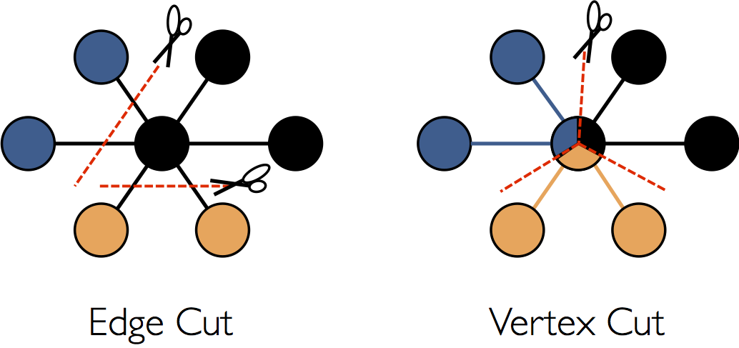
Figure from (Xin, Gonzalez, Franklin, & Stoica, 2013)

Why are Edge-cuts expensive ?

Edge-cuts for partitioning requires random assignment of vertices and edges across all the machines. Thus the communication and storage overhead is proportional to the number of edges cut, and this makes balancing the number of cuts a priority. For most real-world graphs, constructing an optimal edge-cut is cost prohibitive, and most systems use random edge-cuts which achieve appropriate work balance, but nearly worst-case communication overhead.

Vertex-cuts - GraphX’s solution to effective partitioning

An alternative approach which does the opposite of edge-cut — evenly assign edges to machines, but allow vertices to span multiple machines. The communication and storage overhead of a vertex-cut is directly proportional to the sum of the number of machines spanned by each vertex. Therefore, we can reduce communication overhead and ensure balanced computation by evenly assigning edges to machines in a way that minimizes the number of machines spanned by each vertex.

Implementation of Vertex-cut

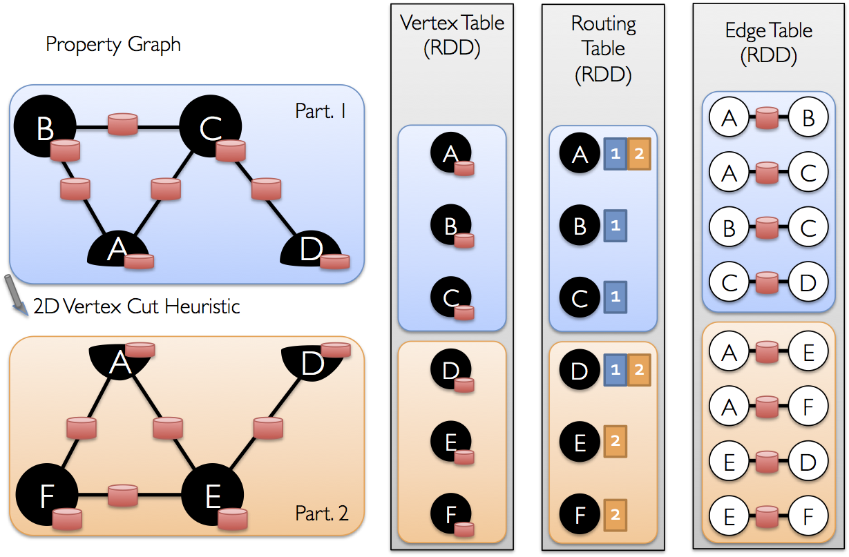
Figure from: https://spark.apache.org/docs/2.0.0-preview/graphx-programming-guide.html

The GraphX RDG structure implements a vertex-cut representation of a graph using three unordered horizontally partitioned RDD tables. These three tables are as follows:

• EdgeTable(pid, src, dst, data): Stores adjacency structure and edge data.
• VertexDataTable(id, data): Stores vertex data. Contains states associated with vertices that are changing in the course of graph computation
• VertexMap/Routing Table(id, pid): Maps vertex ids to the partitions that contain their adjacent edges. Remains static as long as the graph structure doesn’t change.

Execution Models

There are many possible implementations for those programming models. In this section, we will discuss a few different execution models, how the above programming interfaces exploit them, the benefits and limitations of each design and so on. At a very high level, MapReduce, its variants, and Spark all adopt the master/workers model, where the master (or driver in Spark) is responsible for managing data and dynamically scheduling tasks to workers. The master monitors workers’ status, and when failure happens, the master will reschedule the task to another idle worker. However, data in MapReduce (section 2.1) is distributed over clusters and needs to be moved in and out of the disk, and Spark (section 2.2) takes the in-memory processing approach. This practice saves significant I/O operations and thus is much faster than MapReduce. As for fault tolerance, MapReduce uses data persistence and Spark achieves it by using lineage (recomputation for failed task).

As for more declarative querying models, the execution engine needs to take care of query compilation and in the meantime has the opportunity of optimizations. For example, Hive (section 2.3) not only needs a driver the way MapReduce and Spark do, but also has to manage the meta store as well to take advantage of optimization gains from a traditional database like design. SparkSQL (section 2.4) adopts Catalyst framework for SQL optimization which is rule-based and cost-based.

MapReduce execution model

The original MapReduce model is implemented and deployed in Google infrastructure. As described in section 1.1.1, user program defines map and reduce functions and the underlying system manages data partition and schedules jobs across different nodes. Figure 2.1.1 shows the overall flow when the user program calls MapReduce function:

1. Split data. The input files are split into M pieces;
2. Copy processes. The user program creates a master process and the workers. The master picks idle workers to do either map or reduce task;
3. Map. The map worker reads corresponding splits and passes to the map function. The generated intermediate key/value pairs are buffered in memory;
4. Partition. The buffered pairs are written to local disk and partitioned to R regions periodically. Then the locations are passed back to the master;
5. Shuffle. The reduce worker reads from the local disks and groups together all occurrences of the same key together;
6. Reduce. The reduce worker iterates over the grouped intermediate data and calls reduce function on each key and its set of values. The worker appends the output to a final output file;
7. Wake up. When all tasks finish, the master wakes up the user program.

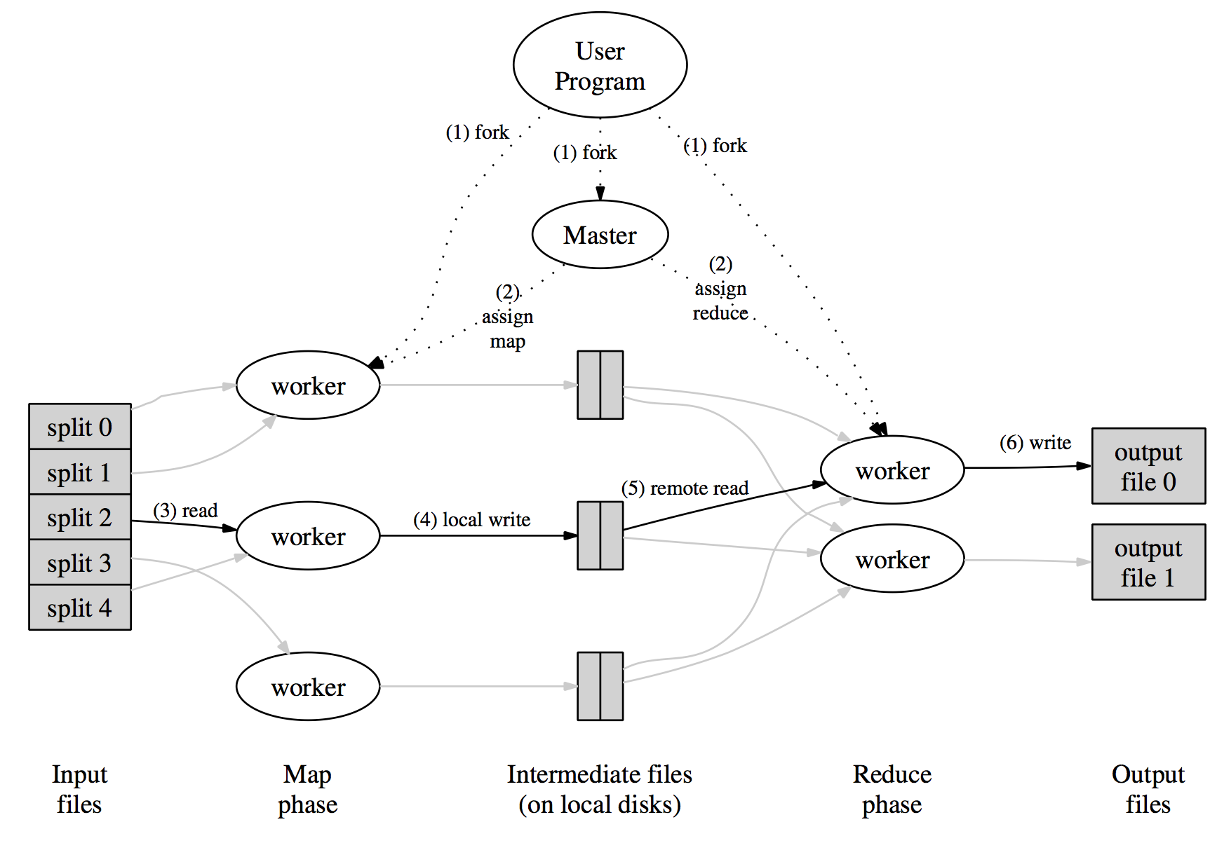
At step 4 and 5, the intermediate dataset is written to the disk by map worker and then read from the disk by reducing worker. Transferring big data chunks over the network is expensive, so the data is stored on local disks of the cluster and the master tries to schedule the map task on the machine that contains the dataset or a nearby machine to minimize the network operation.

Spark execution model

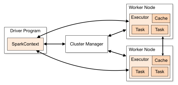
Figure & information (this section) from: http://spark.apache.org/docs/latest/cluster-overview.html

The Spark driver defines SparkContext which is the entry point for any job that defines the environment/configuration and the dependencies of the submitted job. It connects to the cluster manager and requests resources for further execution of the jobs. The cluster manager manages and allocates the required system resources to the Spark jobs. Furthermore, it coordinates and keeps track of the live/dead nodes in a cluster. It enables the execution of jobs submitted by the driver on the worker nodes (also called Spark workers) and finally tracks and shows the status of various jobs running on the worker nodes. A Spark worker executes the business logic submitted by the user by way of the Spark driver. Spark workers are abstracted and are allocated dynamically by the cluster manager to the Spark driver for the execution of submitted jobs. The driver will listen for and accept incoming connections from its executors throughout its lifetime.

Job scheduler optimization

Spark’s job scheduler tracks the persistent RDD’s saved in memory. When an action (count or collect) is performed on an RDD, the scheduler first analyzes the lineage graph to build a DAG of stages to execute. These stages only contain the transformations having narrow dependencies. Outside these stages are the wider dependencies for which the scheduler has to fetch the missing partitions from other workers in order to build the target RDD. The job scheduler is highly performant. It assigns tasks to machines based on data locality or to the preferred machines in the contained RDD. If a task fails, the scheduler re-runs it on another node and also recomputes the stage’s parent is missing.

How are persistent RDD’s memory managed ?

Persistent RDDs are stored in memory as java objects (for performance) or in memory as serialized data (for less memory usage at cost of performance) or on disk. If the worker runs out of memory upon creation of a new RDD, Least Recently Used(LRU) policy is applied to evict the least recently accessed RDD unless its same as the new RDD. In that case, the old RDD is excluded from eviction given the fact that it may be reused again in future. Long lineage chains involving wide dependencies are checkpointed to reduce the time in recovering an RDD. However, since RDDs are read-only, checkpointing is still ok since consistency is not a concern and there is no overhead to manage the consistency as is seen in distributed shared memory.

Hive execution model

The Hive execution model (Thusoo et al., 2010) is composed of the following important components (and as shown in the below Hive architecutre diagram below):

• Driver: Similar to the Drivers of Spark/MapReduce application, the driver in Hive handles query submission & its flow across the system. It also manages the session and its statistics.

• Metastore – A Hive meta store stores all information about the tables, their partitions, schemas, columns and their types, etc. enabling transparency of data format and its storage to the users. It, in turn, helps in data exploration, query compilation, and optimization. Criticality of the Matastore for managing the structure of Hadoop files requires it to be updated on a regular basis.

• Query Compiler – The Hive Query compiler is similar to any traditional database compilers. it processes the query in three steps:
• Parse: In this phase, it uses Antlr (A parser generator tool) to generate the Abstract syntax tree (AST) of the query.

• Transformation of AST to DAG (Directed acyclic graph): In this phase, it generates a logical plan and does a compile type checking. The logical plan is generated using the metadata (stored in Metastore) information of the required tables. It can flag errors if any issues found during the type checking.

• Optimization: Optimization forms the core of any declarative interface. In the case of Hive, optimization happens through chains of transformation of DAG. A transformation could include even a user defined optimization and it applies an action on the DAG only if a rule is satisfied. Every node in the DAG implements a special interface called as Node interface which makes it easy for the manipulation of the operator DAG using other interfaces like GraphWalker, Dispatcher, Rule, and Processor. Hence, by transformation, we mean walking through a DAG and for every Node we encounter we perform a Rule satisfiability check. If a Rule is satisfied, a corresponding processor is invoked. A Dispatcher maintains a list of Rule to Processor mappings.

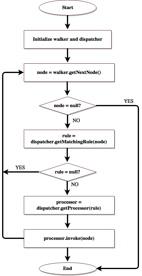
Figure to depict the transformation flow during optimization, from: (Thusoo et al., 2010)

• Execution Engine: Execution Engine finally executes the tasks in order of their dependencies. A MapReduce task first serializes its part of the plan into a plan.xml file. This file is then added to the job cache and mappers and reducers are spawned to execute relevant sections of the operator DAG. The final results are stored to a temporary location and then moved to the final destination (in the case of say an INSERT INTO query).

Summarizing the flow

Hive architecture diagram

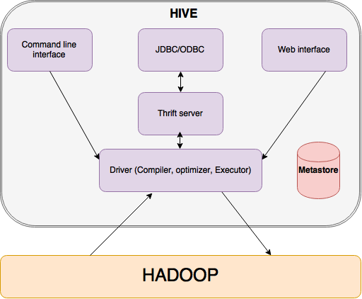
The query is first submitted via CLI/the web UI/any other interface. The query undergoes all the compiler phases as explained above to form an optimized DAG of MapReduce and its tasks which the execution engine executes in its correct order using Hadoop.

Some of the important optimization techniques in Hive are:

• Column Pruning - Consider only the required columns needed in the query processing for projection.
• Predicate Pushdown - Filter the rows as early as possible by pushing down the predicates. It is important that unnecessary records are filtered first and transformations are applied to only the needed ones.
• Partition Pruning - Predicates on partitioned columns are used to prune out files of partitions that do not satisfy the predicate.
• Map Side Joins - Smaller tables in the join operation can be replicated in all the mappers and the reducers.
• Join Reordering - Reduce “reducer side” join operation memory by keeping only smaller tables in memory. Larger tables need not be kept in memory.
• Repartitioning data to handle skew in GROUP BY processing can be achieved by performing GROUP BY in two MapReduce stages. In first stage data is distributed randomly to the reducers and partial aggregation is performed. In the second stage, these partial aggregations are distributed on GROUP BY columns to different reducers.
• Similar to combiners in MapReduce, hash based partial aggregations in the mappers can be performed to reduce the data that is sent by the mappers to the reducers. This helps in reducing the amount of time spent in sorting and merging the resulting data.

SparkSQL execution model

SparkSQL (Armbrust et al., 2015) execution model leverages Catalyst framework for optimizing the SQL before submitting it to the Spark Core engine for scheduling the job. A Catalyst is a query optimizer. Query optimizers for MapReduce frameworks can greatly improve performance of the queries developers write and also significantly reduce the development time. A good query optimizer should be able to optimize user queries, extensible for user to provide information about the data and even dynamically include developer defined specific rules.

Catalyst leverages the Scala’s functional language features like pattern matching and runtime meta programming to allow developers to concisely specify complex relational optimizations.

Catalyst includes both rule-based and cost-based optimization. It is extensible to include new optimization techniques and features to Spark SQL and also let developers provide data source specific rules. Catalyst executes the rules on its data type Tree - a composition of node objects where each node has a node type (subclasses of TreeNode class in Scala) and zero or more children. Node objects are immutable and can be manipulated. The transform method of a Tree applies pattern matching to match a subset of all possible input trees on which the optimization rules needs to be applied.

Hence, in Spark SQL, transformation of user queries happens in four phases:

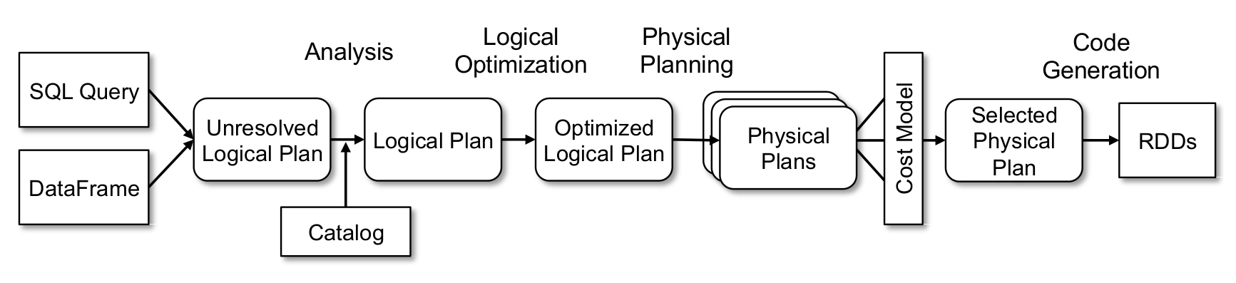
Figure from: (Armbrust et al., 2015)

Analyzing a logical plan to resolve references: In the analysis phase a relation either from the abstract syntax tree (AST) returned by the SQL parser or from a DataFrame is analyzed to create a logical plan out of it, which is still unresolved (the columns referred may not exist or may be of wrong datatype). The logical plan is resolved using using the Catalyst’s Catalog object (tracks the table from all data sources) by mapping the named attributes to the input provided, looking up the relations by name from catalog, by propagating and coercing types through expressions.

Logical plan optimization: In this phase, several of the rules like constant folding, predicate push down, projection pruning, null propagation, boolean expression simplification are applied on the logical plan.

Physical planning: In this phase, Spark generates multiples physical plans out of the input logical plan and chooses the plan based on a cost model. The physical planner also performs rule-based physical optimizations, such as pipelining projections or filters into one Spark map operation. In addition, it can push operations from the logical plan into data sources that support predicate or projection pushdown.

Code Generation: The final phase generates the Java byte code that should run on each machine. Catalyst transforms the Tree which is an expression in SQL to an AST for Scala code to evaluate, compile and run the generated code. A special scala feature namely quasiquotes aid in the construction of abstract syntax tree (AST).

Big Data Ecosystem

Hadoop Ecosystem

Apache Hadoop is an open-sourced framework that supports distributed processing of large dataset. It involves dozens of projects, all of which are listed here. In this section, it is also important to understand the key players in the system, namely two parts: the Hadoop Distributed File System (HDFS) and the open-sourced implementation of MapReduce model - Hadoop.

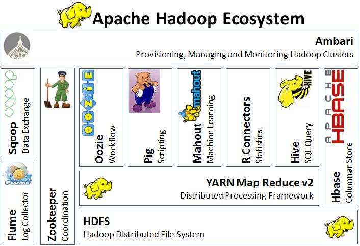
Figure from http://thebigdatablog.weebly.com/blog/the-hadoop-ecosystem-overview

HDFS forms the data management layer, which is a distributed file system designed to provide reliable, scalable storage across large clusters of unreliable commodity machines. The idea was inspired by GFS (Ghemawat, Gobioff, & Leung, 2003). Unlike closed GFS, HDFS is open-sourced and provides various libraries and interfaces to support different file systems, like S3, KFS etc.

To satisfy different needs, big companies like Facebook and Yahoo developed additional tools. Facebook’s Hive, as a warehouse system, can provide more declarative programming interface and translate to Hadoop jobs. Yahoo’s Pig platform is an ad-hoc analysis tool that can structurize HDFS objects and support operations like grouping, joining and filtering.

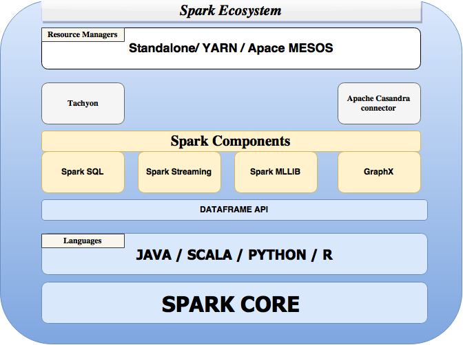
Spark ecosystem

Apache Spark’s rich ecosystem benefits from other resource management systems like (Hindman et al., 2011), Yarn (Vavilapalli et al., 2013), and several major components that have been already discussed in this article like Spark-core, SparkSQL, GraphX.

In this section we will discuss the remaining important libraries and systems which help Spark deliver high performance.

Spark Streaming - A Spark component for streaming workloads

Spark achieves fault tolerant, high throughput data streaming workloads in real-time through a light weight Spark Streaming API. Spark streaming is based on Discretized Streams model. (Zaharia, Das, Li, Shenker, & Stoica, 2012) Spark Streaming processes streaming workloads as a series of small batch workloads by leveraging the fast scheduling capacity of Apache Spark Core and fault tolerance capabilities of a RDD. A RDD in here represents each batch of streaming data and transformations are applied on the same. Data source in Spark Streaming could be from many a live streams like Twitter, Apache Kafka (Kreps, Narkhede, Rao, & others, 2011), Akka Actors, IoT Sensors, Apache Flume, etc. Spark streaming also enables unification of batch and streaming workloads and hence developers can use the same code for both batch and streaming workloads. It supports the integration of streaming data with historical data.

Apache Mesos

Apache Mesos (Hindman et al., 2011) is an open source heterogenous cluster/resource manager developed at the University of California, Berkley and used by companies such as Twitter, Airbnb, Netflix etc. for handling workloads in a distributed environment through dynamic resource sharing and isolation. It aids in the deployment and management of applications in large-scale clustered environments. Mesos abstracts node allocation by combining the existing resources of the machines/nodes in a cluster into a single pool and enabling fault-tolerant elastic distributed systems. Variety of workloads can utilize the nodes from this single pool voiding the need of allocating specific machines for different workloads. Mesos is highly scalable, achieves fault tolerance through Apache Zookeeper (Hunt, Konar, Junqueira, & Reed, 2010) and is a efficient CPU and memory-aware resource scheduler.

Alluxio/Tachyon

Alluxio/Tachyon (Li, Ghodsi, Zaharia, Shenker, & Stoica, 2014) is an open source memory-centric distributed storage system that provides high throughput writes and reads enabling reliable data sharing at memory-speed across cluster jobs. Tachyon can integrate with different computation frameworks, such as Apache Spark and Apache MapReduce. In the big data ecosystem, Tachyon fits between computation frameworks or jobs like spark or mapreducce and various kinds of storage systems, such as Amazon S3, OpenStack Swift, GlusterFS, HDFS, or Ceph. It caches the frequently read datasets in memory, thereby avoiding going to disk to load every dataset. In Spark RDDs can automatically be stored inside Tachyon to make Spark more resilient and avoid GC overheads.

References

1. Armbrust, M., Das, T., Davidson, A., Ghodsi, A., Or, A., Rosen, J., … Zaharia, M. (2015). Scaling spark in the real world: performance and usability. Proceedings of the VLDB Endowment, 8(12), 1840–1843.
2. Armbrust, M., Xin, R. S., Lian, C., Huai, Y., Liu, D., Bradley, J. K., … others. (2015). Spark sql: Relational data processing in spark. In Proceedings of the 2015 ACM SIGMOD International Conference on Management of Data (pp. 1383–1394). ACM.
3. Bu, Y., Howe, B., Balazinska, M., & Ernst, M. D. (2010). HaLoop: efficient iterative data processing on large clusters. Proceedings of the VLDB Endowment, 3(1-2), 285–296.
4. Chambers, C., Raniwala, A., Perry, F., Adams, S., Henry, R. R., Bradshaw, R., & Weizenbaum, N. (2010). FlumeJava: easy, efficient data-parallel pipelines. In ACM Sigplan Notices (Vol. 45, pp. 363–375). ACM.
5. Ching, A., Edunov, S., Kabiljo, M., Logothetis, D., & Muthukrishnan, S. (2015). One trillion edges: graph processing at Facebook-scale. Proceedings of the VLDB Endowment, 8(12), 1804–1815.
6. Dean, J., & Ghemawat, S. (2008). MapReduce: simplified data processing on large clusters. Communications of the ACM, 51(1), 107–113.
7. Ekanayake, J., Li, H., Zhang, B., Gunarathne, T., Bae, S.-H., Qiu, J., & Fox, G. (2010). Twister: a runtime for iterative mapreduce. In Proceedings of the 19th ACM International Symposium on High Performance Distributed Computing (pp. 810–818). ACM.
8. Ghemawat, S., Gobioff, H., & Leung, S.-T. (2003). The Google file system. In ACM SIGOPS operating systems review (Vol. 37, pp. 29–43). ACM.
9. Gonzalez, J. E., Low, Y., Gu, H., Bickson, D., & Guestrin, C. (2012). Powergraph: Distributed graph-parallel computation on natural graphs. In Presented as part of the 10th USENIX Symposium on Operating Systems Design and Implementation (OSDI 12) (pp. 17–30).
10. Hindman, B., Konwinski, A., Zaharia, M., Ghodsi, A., Joseph, A. D., Katz, R. H., … Stoica, I. (2011). Mesos: A Platform for Fine-Grained Resource Sharing in the Data Center. In NSDI (Vol. 11, pp. 22–22).
11. Hunt, P., Konar, M., Junqueira, F. P., & Reed, B. (2010). ZooKeeper: Wait-free Coordination for Internet-scale Systems. In USENIX Annual Technical Conference (Vol. 8, p. 9).
12. Isard, M., Budiu, M., Yu, Y., Birrell, A., & Fetterly, D. (2007). Dryad: distributed data-parallel programs from sequential building blocks. In ACM SIGOPS Operating Systems Review (Vol. 41, pp. 59–72). ACM.
13. Kreps, J., Narkhede, N., Rao, J., & others. (2011). Kafka: A distributed messaging system for log processing. In Proceedings of the NetDB (pp. 1–7).
14. Li, H., Ghodsi, A., Zaharia, M., Shenker, S., & Stoica, I. (2014). Tachyon: Reliable, memory speed storage for cluster computing frameworks. In Proceedings of the ACM Symposium on Cloud Computing (pp. 1–15). ACM.
15. Malewicz, G., Austern, M. H., Bik, A. J. C., Dehnert, J. C., Horn, I., Leiser, N., & Czajkowski, G. (2010). Pregel: a system for large-scale graph processing. In Proceedings of the 2010 ACM SIGMOD International Conference on Management of data (pp. 135–146). ACM.
16. Okcan, A., & Riedewald, M. (2011). Processing theta-joins using MapReduce. In Proceedings of the 2011 ACM SIGMOD International Conference on Management of data (pp. 949–960). ACM.
17. Olston, C., Reed, B., Srivastava, U., Kumar, R., & Tomkins, A. (2008). Pig latin: a not-so-foreign language for data processing. In Proceedings of the 2008 ACM SIGMOD international conference on Management of data (pp. 1099–1110). ACM.
18. Pike, R., Dorward, S., Griesemer, R., & Quinlan, S. (2005). Interpreting the data: Parallel analysis with Sawzall. Scientific Programming, 13(4), 277–298.
19. Shvachko, K., Kuang, H., Radia, S., & Chansler, R. (2010). The hadoop distributed file system. In 2010 IEEE 26th symposium on mass storage systems and technologies (MSST) (pp. 1–10). IEEE.
20. Tarau, P. (2014). Bulk synchronous model. Retrieved from http://www.cse.unt.edu/ tarau/teaching/parpro/papers/Bulk%20synchronous%20parallel.pdf
21. Thusoo, A., Sarma, J. S., Jain, N., Shao, Z., Chakka, P., Anthony, S., … Murthy, R. (2009). Hive: a warehousing solution over a map-reduce framework. Proceedings of the VLDB Endowment, 2(2), 1626–1629.
22. Thusoo, A., Sarma, J. S., Jain, N., Shao, Z., Chakka, P., Zhang, N., … Murthy, R. (2010). Hive-a petabyte scale data warehouse using hadoop. In 2010 IEEE 26th International Conference on Data Engineering (ICDE 2010) (pp. 996–1005). IEEE.
23. Valiant, L. G. (1990). A bridging model for parallel computation. Communications of the ACM, 33(8), 103–111.
24. Vavilapalli, V. K., Murthy, A. C., Douglas, C., Agarwal, S., Konar, M., Evans, R., … others. (2013). Apache hadoop yarn: Yet another resource negotiator. In Proceedings of the 4th annual Symposium on Cloud Computing (p. 5). ACM.
25. Xin, R. S., Gonzalez, J. E., Franklin, M. J., & Stoica, I. (2013). Graphx: A resilient distributed graph system on spark. In First International Workshop on Graph Data Management Experiences and Systems (p. 2). ACM.
26. Yu, Y., Isard, M., Fetterly, D., Budiu, M., Erlingsson, Ú., Gunda, P. K., & Currey, J. (2008). DryadLINQ: A System for General-Purpose Distributed Data-Parallel Computing Using a High-Level Language. In OSDI (Vol. 8, pp. 1–14).
27. Zaharia, M., Chowdhury, M., Franklin, M. J., Shenker, S., & Stoica, I. (2010). Spark: cluster computing with working sets. HotCloud, 10, 10–10.
28. Zaharia, M., Das, T., Li, H., Shenker, S., & Stoica, I. (2012). Discretized streams: an efficient and fault-tolerant model for stream processing on large clusters. In Presented as part of the.
29. Zhang, Y., Gao, Q., Gao, L., & Wang, C. (2012). imapreduce: A distributed computing framework for iterative computation. Journal of Grid Computing, 10(1), 47–68.