Large Scale Streaming Processing

The previous chapter discusses the large scale batch processing system, where the computation involves the pieces of data stored across the distributed file system. Those systems satisfy the requirements such as scalability and fault-tolerance for applications that deal with “big data” stored in a distributed way. Batch processing systems are suitable for processing static datasets, where the input data does not change overtime during the whole process, thus the system can distribute the computation and perform synchronization assuming the inputs would stay the same during the whole computation. In such static model, the processing system can first pull data from the disk, and then perform the computation over the pulled data. However, a large number of networking applications are not static, instead, the data is constantly in motion, and the inputs would be provided as stream, as new data constantly arrives. In the stream model, data is pushed to the processor. This fundamental difference makes the traditional batch processing system un-suitable for streaming applications, as even the slightest change in the dataset would require the batch processor to pull the whole dataset and perform the computation again. Thus in this chapter, we would introduce the history and systems that are created for the streaming processing.

There are many challenges for implementing large scale streaming processing system. Similar to large scale batch processing systems, large scale streaming systems also have to deal with consistency and fault-tolerance due to the distributed nature of those systems. Moreover, latency at the scale of several minutes is at most a nuisance in batch processing while latency is not as tolerable in large streaming processing.

Despite those challenges, there are many active research and productions in the stream processing area, and we want to answer the following questions in this article:

1. What are the earliest ideas of stream processing? Why would people want to analyze a stream of data?
2. What exactly is a stream? How is it implemented in real systems?
3. What are the systems that are built for large scale stream processing, and what are the differences between them?
4. What are the systems that are being used by companies for their applications? Do they build their own system or do they use existing systems?

Data in constant motion

Computing data stream has long been studied in the area of Theory of Computing. Assume we have a sequence of elements, and we want to compute the frequency moments of the data (i.e., count how many of each of the distinct data appear in the sequence). To do that, we could maintain a full histogram on the data, a counter for each data value. However, the memory that we have is not unlimited, thus we can not gather every data, we can then use randomized algorithms for approximating the frequency moments with limited resource (Alon, Matias, & Szegedy, 1996). Thus analyzing the stream using random algorithm was because of the lack of computation resources.

Besides randomized processing on the data sequence, systems were also being developed to deal with the input data that is not static and predictable. Instead of dealing with the lack of resources, those projects were mostly motivated by the fact that in emerging networked environments, the value of the ever increasing amount of data is realized only within the time that it is needed. TelegraphCQ (Chandrasekaran et al., 2003) is one example among those earliest such systems, which aims at meeting the challenges that arise in handling large streams of continuous queries over high-volume, high-variable data. In contrast to traditional view that data can be found statically in known locations, the authors of TelegraphCQ realized that data becomes fluid and being constantly moving and changing, thus the traditional database can “pull” data from the storage while data is being “pushed” into the query processor in case of processing stream. The examples of applications that use this data in motion include: event-based processing where the system would react to some special data received or when some event happens (e.g., at a certain time), and query processing over streaming data sources such as network monitoring. TelegraphCQ is one example of the systems that can query processing over data stream.

The fundamental difference between TelegraphCQ and other traditional query system is its view of input data. Instead of handling a query with detailed static data, TelegraphCQ has to react to the newly arrived data and process the queries on-the-fly. In order to always react, the query needs to be always running, so TelegraphCQ runs continuous queries, where the queries are constantly running and as new data arrives, the processor routes it to the set of active queries that are listening. TelegraphCQ also uses shared processing to avoid the overhead of processing each query individually, in order to avoid blocking and having to interrupt the dataflow, data should be processed simultaneously by all the queries that require this dataflow. In TelegraphCQ, those queries with such commonality can be combined together to improve the performance.

TelegraphCQ shows the importance of modeling data as stream and how can we process such data stream, however it was only implemented in a non-distributed prototype.

Beyond TelegraphCQ, there are systems that were built for continuously querying on large scale streaming data. For example, PipelineDB (“PipelineDB,” n.d.) is a system that was designed to run SQL queries continuously on streaming data, where the output of those continuous queries is stored in regular tables which can be queried like any other table. PipelineDB can reduce the cardinality of its input streams by performing different filtering or aggregations on stream once the continuous queries read the raw data, and only the needed information would then be persisted to disk (i.e., the raw data is then discarded). By doing this, PipelineDB can process large volumes of data very efficiently using relatively small number of resources.

As we described before, stream processing is not only query processing. Apache Flink (“Apache Flink,” n.d.) is a system that supports both event-based processing and query processing. Each program in Flink is a streaming dafalow consisting of streams and transformation operators, the stream of data in a streaming dataflow can come from multiple sources (i.e., producers) and travel to one or more sinks (i.e., consumers). The stream of data would get transformed when traveling through the operators, where the computations happen. In order to distribute the work, streams are split into stream partitions and operators are split into operator subtasks in Flink where each subtask executes independently.

What is event-based processing in Flink then? Unlike batch processing, to aggregate a event is more subtle in stream processing, for example we can not count the element in a stream since it is generally unbounded. Instead, Flink enables event-based processing with the notion of time and windows. For example, we can specify something like ‘count over 5 minutes window’. Besides time-based windows, Flink also supports count-based windows, and operations like ‘do something when the 100th element arrives’. Flink has different notions of time such as event time when an event was created and processing time which is when the operator performs a time-based operation. The time are then used internally to keep the order and state for each event and also used by the windowing logic. The flexible streaming windows can then be transformed to flexible triggering condition which makes event-based processing possible in Flink.

We just very briefly introduced PipelineDB and Apache Flink here, and there are many other systems that can perform stream processing in large scale and we would look into few examples in detail in section 3.

How to represent data stream

Why would we need to process data stream in a large scale? I will use an example to illustrate the idea. For example, assume you are Twitter, and you have a constant feed of user’s comments and posts, you want to find out what is the most trending topic right now that people are talking about, and your advertisement team want to follow on that. You can store all the posts that happened during the day from 12:01 a.m to 11:59 p.m in a large file system and then run a batch Spark (Zaharia et al., 2012) job to analyze them. The Spark job itself may again probably take several hours, but after all these works, the trending topic comes out from your analysis might be useless since it might not be hot anymore. Thus we want a stream processing system that can take the constant stream of posts from all different sources as input and output the result with low latency (i.e. before it becomes useless).

Before dive into the details of the large scale processing, we would first introduce a few concepts: producer, processor and consumer based on the example.

• The producer is where the data stream comes from, it would be a user who is tweeting.
• The consumer is where the results are needed, the advertisement team would be the consumer.
• The processor is then the magical component that takes the stream and produces the results.

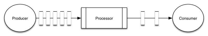
The producers and consumers are fairly straight forward, it is the processor that are being discussed in this chapter.

In this section, we would first illustrate what is the stream (i.e. the tuples between components) that the producers are giving to the processor, which is the component between producers and processors-the data stream.

We have been talking about the stream of data, but this is a bit under-specified, since the data can be collected from many producers (i.e. different users), how do we combine those data into actual streams and send the them to the processors? What does a data stream really look like?

A natural view of a data stream can be an infinite sequence of tuples reading from a queue. However, a traditional queue would not be sufficient in large scale system since the consumed tuple might got lost or the consumer might fail thus it might request the previous tuple after a restart. Furthermore, since the processing power for a single machine is limited, we want several machines to be able to read from the same queue, thus they can work on the stream in parallel. The alternative queue design is then a multi-consumer queue, where a pool of readers may read from a single queue and each record goes to one of them. In a traditional multi-consumer queue, once a consumer reads the data out, it is gone. This would be problematic in a large stream processing system, since the messages are more likely to be lost during transmission, and we want to keep track of what are the data that are successfully being consumed and what are the data that might be lost on their way towards the consumer. Thus we need a little fancier queue to keep track of what has been consumed, in order to be resilient in the face of packet loss or network failure.

A naive approach to attempting to handle lost messages or failures could be to record the message upon sending it, and to wait for the acknowledgement from the receiver. This simple method is a pragmatic choice since the storage in many messaging systems are scarce resources, the system want to free the data immediately once it knows it is consumed successfully thus to keep the queue small. However, getting the two ends to come into agreement about what has been consumed in not a trivial problem. Acknowledgement fixes the problem of losing messages, because if a message is lost, it would not be acknowledged thus the data is still in the queue and can be sent again, this would ensure that each message is processed at least once, however, it also creates new problems. First problem is the receiver might successfully consumed the message m1 but fail to send the acknowledgment, thus the sender would send m1 again and the receiver would process the same data twice. Another problem is memory consumption, since the sender has now to keep track of every single messages being sent out with multiple stages, and only free them when acknowledged.

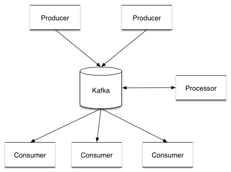
Apache Kafka (“Apache Kafka,” n.d.) handles this differently to achieve better performance. Apache Kafka is a distributed streaming platform, where the producer, processor and consumers can all subscribe to, and create/read the stream they need from, one can think of Kafka as the stream between all components in a stream processing system. Records in Kafka are grouped in topics, where each topic is a category to which this record is published. Each topic is then divided into several partitions, where one topic can always have multi-subscriber and each partition has one reader at a time. Each record is assigned with a offset that uniquely identifies it in that partition. By doing this Kafka can ensure that the only reader of that partition and consumes the data in order. Since there are many partitions of each topic, Kafka balances the load over many consumer instances by assigning different partitions to them. This makes the state about what has been consumed very small, just one number (i.e. the offset) for each partition, and by periodically checkpointing, the equivalent of message acknowledgements becomes very cheap. Kafka retains all published records whether they have been consumed or not during their configurable retention period, this also allows consumers to rewind the stream and replay everything from the point of interest by going back to the specific offset. For example, if the user code has a bug which is discovered later, the user can re-consume those messages from the previous offset once the bug is fixed while ensuring that the processed events are in the order of their origination, or the user can simply start computing with the latest records from “now”.

With the notions of topics and partitions, Kafka guarantees that the total order over records within a partition, and multiple consumers can subscribe to a single topic which would increase the throughput. If a strong guarantee on the ordering of all records in a topic is needed, the user can simply put all records in this topic into one partition.

Those features of Apache Kafka make it a very popular platform used by many stream processing systems, and we can think of the stream as Apache Kafka in the rest of this article.

How to process data stream

Now we know what the stream looks like and how do we ensure that the data in the stream are successfully processed. We would then talk about the processors that consume the data stream. There are two main approaches in processing data stream. The first approach is the continuous queries model, similar to TelegraphCQ, where the queries keep running and the arrival of data initiates the processing. Another approach is micro-batching, where the streaming computation becomes a series of stateless, deterministic batch computations on batch of stream, where certain timer would trigger the processing on the batch in those systems. We would discuss Apache Storm as one example for the fist design and Spark Streaming, Naiad, and Google Dataflow as examples of the second approach. These systems not only differ in how they process stream, but also how they ensure fault-tolerance which is one of the most important aspects of large scale distributed system.

Continuous queries (operators) on each tuple

Apache Storm

After MapReduce, Hadoop, and the related batch processing system came out, the data can be processed at scales previously unthinkable. However, as we stated before, large scale stream processing becomes more and more important for many businesses. Apache Storm (“Apache Storm,” n.d.) is actually one of the first system that can be described as “Hadoop of stream processing” that feed the needs. Users can process messages in a way that doesn’t lose data and also scalable with the primitives provided by Storm.

In Storm, the logic of every processing job is described as a Storm topology. A Storm topology in Storm can be think of as a MapReduce job in Hadoop, the difference is that a MapReduce job will finish eventually but a Storm topology will run forever. There are three components in the topology: stream, spouts and bolts.

In Storm, a stream is a unbounded sequence of tuples, tuples can contain arbitrary types of data, which also related to the core concept of Storm: process the tuples in a stream.

The next abstraction in a topology is spout. A spout is a source of streams. For example, a spout may read tuples off of a Kafka queue as we discussed before and emit them as a stream.

A bolt is where the processing really take place, it can take multiple streams as input and produce multiple streams as output. Bolts are where the logic of the topology are implemented, they can run functions, filter data, compute aggregations and so forth.

A topology is then arbitrary combination of the three components, where spouts and bolts are the vertices and streams are the edges in the topology.

TopologyBuilder builder = new TopologyBuilder();        
builder.setSpout("words", new TestWordSpout(), 10);        
builder.setBolt("exclaim1", new ExclamationBolt(), 3)
        	.shuffleGrouping("words");
builder.setBolt("exclaim2", new ExclamationBolt(), 5)
            .shuffleGrouping("words")
            .shuffleGrouping("exclaim1");

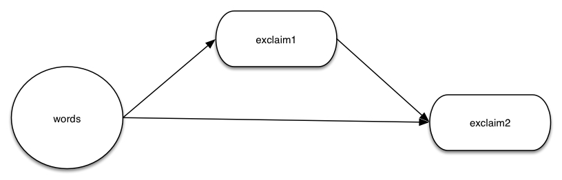
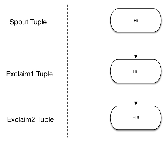
Here is how we can build a simple topology which contains a spout and two bolts, where the spout emits words and each bolt would append exclamation "!" to its input. The exclaim1 bolt is connected to the spout while the exclaim2 bolt is connected to both the spout and exclaim2 specified by ‘Grouping’, and we will show what ‘shuffle grouping’ means in the next paragraph. The nodes are arranged as shown in the graph. For example if the bolt emits the tuple ["Hi"], if it travels from exclaim1 to exclaim2, then exclaim2 would emit the word ["Hi!!"].

Since all the works are distributed, any given vertex is not necessarily running on a single machine, instead they can be spread on different workers in the cluster. The parameters 10, 3 and 5 in the example code actually specify the amount of parallelism the user wants. Storm also provides different stream grouping schemes for users to determine which vertex should be consuming the output stream from a given vertex. The grouping method can be shuffle grouping as shown in our example, where the tuples from the output stream will be randomly distributed across this bolt’s consumers in a way such that each consumer is guaranteed to get an equal number of tuples. Another example would be fields grouping, where the tuples of the stream is partitioned by the fields specified in the grouping, the tuples with the same value in that field would always go to the same bolt.

A natural question to ask here is what if something goes wrong for example: what if a single tuple gets lost? One might think that Storm maintains a queue similar to what we discussed before to ensure that every tuple is processed at least once. In fact, Storm does not keep such queues internally, the reason might be that there would be so many states to maintain if it needs to construct such queue for every edge. In stead, Storm maintains a directed acyclic graph (DAG) for every single tuple, where each DAG contains the information of this tuple as how the original tuple is split among different workers. Storm uses the DAG to track each tuple, if the tuple fails to be processed, then the system would retry the tuple from the spout again.

There might be two concerns here. The first is how can Storm track every DAG efficiently and scalably, would it actually use more resources than just maintain the queues? The second concern is starting all the way from spout again instead of the intermediate queue seems taking a step backwards. For the first concern, Storm actually uses a very efficient algorithm to create the DAG of each tuple, it would take at most 20 bytes for any tuple even if the DAG contains trillions of tuples in it. For the second concern, if we look at the guarantees provided by both techniques, tracking DAG and intermediate queues, they are actually the same. They both guarantee that each tuple is processed at least once, so there are no fundamental differences between them.

Thus as shown before, Storm can guarantee the primitives, it can process a stream of data, distribute the work among multiple workers and guarantee each tuple in the stream is processed.

Micro-batch

We have seen Apache Storm as a stream processing system that has the guarantees needed by such system. However, the core of Storm is to process stream at a granularity of each tuple. Sometimes such granularity is unnecessary, for the Twitter example that we had before, maybe we are only interested in the stream of tuples that came within a 5 minutes interval, with Storm, such specification can only be set on top of the system while one really want a convenient way to express such requirement within the system itself. In the next section, we would introduce several other stream processing systems, all of them can act on data stream in real time at large scale as Storm, but they provide more ways for the users to express how they want the tuples in the stream to be grouped and then processed. We refer to grouping the tuples before processing them as putting them into small micro-batches, and the processor can then provide results by working on those batches instead of single tuple.

Spark Streaming

The Spark streaming (Zaharia, Das, Li, Shenker, & Stoica, 2012) system is built upon Apache Spark, a system for large-scale parallel batch processing, which uses a data-sharing abstraction called ‘Resilient Distributed Datasets’ or RDDs to ensure fault-tolerance while achieve extremely low latency. The challenges with ‘big data’ stream processing were long recovery time when failure happens, and the the stragglers might increase the processing time of the whole system. Spark streaming overcomes those challenges by a parallel recovery mechanism that improves efficiency over traditional replication and backup schemes, and tolerate stragglers.

The challenge of the fault-tolerance comes from the fact that the stream processing system might need hundreds of nodes, at such scale, two major problems are faults and stragglers. Some system use continuous processing model such as Storm, in which long-running, stateful queries receive each tuple, update its state and send out the result tuple. While such model is natural, it also makes difficult to handle faults. As shown before Storm uses upstream backup, where the messages are buffered and replayed if a message fail to be processed. Another approach for fault-tolerance used by previous system is replication, where there are two copies of everything. The first approach takes long time to recovery while the latter one costs double the storage space. Moreover, neither approach handles stragglers. In the first approach, a straggler must be treated as a failure which incurs a costly recovery while the straggler would slow down both replicas because of the use of synchronization protocols to coordinate replicas in the second approach.

Spark streaming overcomes these challenges by a new stream processing model-instead of running long-lived queries, it divided a stream into a series of batched tuples on small time intervals, then launch a Spark job to process on the batch. Each computation is deterministic given the input data in that time interval, and this also makes parallel recovery possible, when a node fails, each node in the cluster works to recompute part of the lost node’s RDDs. Spark streaming can also recover from straggler in a similar way.

D-stream is the Spark streaming abstraction, and in the D-stream model, a streaming computation is treated as series of deterministic batch computations on small time intervals. Each batch of the stream is stored as RDDs, and the result after processing this RDD also be stored as RDDs. A D-stream is a sequence of RDDs that can be transformed into new D-streams. For example, a stream can be divided into one second batches, to process the events in second s, Spark streaming would first launch a map job to process the events happened in second s and it would then launch a reduce job that take both this mapped result the reduced result of data s - 1. Thus each D-stream can turn into a sequence of RDDs, and the lineage (i.e., the sequence of operations used to build it) of the D-streams are tracked for recovery. If a node fails, it would recover the lost RDD partitions by re-running the operations that used to create them. The re-computation can be ran in parallel on separate nodes since the lineage is distributed, and the work on straggler can be re-ran the same way.

val ssc = new StreamingContext(conf, Seconds(1))      
val lines = ssc.socketTextStream("localhost", 9999)        
val words = lines.flatMap(_.split(" "))
val pairs = words.map(word => (word, 1))
val wordCounts = pairs.reduceByKey(_ + _)
wordCounts.print()

Let’s look at an example of how we can count the word received from a TCP socket with Spark streaming. We first set the processing interval to be 1 second, and we will create a D-stream lines that represents the streaming data received from the specific TCP socket. Then we split the lines by space into words, now the stream of words is represented as the words D-stream. The words stream is further mapped to a D-stream of pairs, which is then reduced to count the number of words in each batch of data.

Spark streaming handles the slow recovery and straggler issue by dividing stream into small batches on small time intervals and using RDDs to keep track of how the result of certain batched stream is computed. This model makes handling recovery and straggler easier because the computation can be ran in parallel by re-computing the result while RDDs make the process fast.

Structured Streaming

Besides Spark streaming, Apache Spark recently added a new higher-level API, Structured Streaming(“Structured Streaming,” n.d.), which is also built on top of the notion of RDDs while makes a strong guarantee that the output of the application is equivalent to executing a batch job on a prefix of data at any time, which is also known as prefix integrity. Structured Streaming makes sure that the output tables are always consistent with all the records in a prefix of the data, thus the out-of-order data is easy to identify and can simply be used to update its respective row in the table. Structured Streaming provides a simple API where the users can just specify the query as if it were a static table, and the systems would automatically convert this query to a stream processing job.

// Read data continuously from an S3 location
val inputDF = spark.readStream.json("s3://logs")
 
// Do operations using the standard DataFrame API and write to MySQL
inputDF.groupBy($"action", window($"time", "1 hour")).count()
       .writeStream.format("jdbc")
       .start("jdbc:mysql//...")

The programming model of Structured Streaming views the latest data as newly appended rows in an unbounded table, every trigger interval, new rows would be added to the existing table which would eventually update the output table. The event-time then becomes nature in this view, since each event from producers is a row where the even-time is just a column value in this row, which then makes window-based aggregations become simply grouping on the event-time column.

Unlike other systems where users have to specify how to aggregate the records when outputing, Structured Streaming would take care of updating the result table when there is new data, users can then just specify different modes to decide what gets written to the external storage. For example in Complete Mode, the entire updated result table would be written to external storage while in Update Mode, only the rows that were updated in the result table will be written out.

Naiad

Naiad (Murray et al., 2013) is another distributed system for executing data stream which is developed by Microsoft. Naiad combines the benefits of high throughput of batch processors and the low latency of stream processors by its computation model called timely dataflow that enables dataflow computations with timestamps.

The timely dataflow, like topology described in Storm, contains stateful vertices that represent the nodes that would compute on the stream. Each graph contains input vertices and output vertices, which are responsible for consuming or producing messages from external sources. Every message being exchanged is associated with a timestamp called epoch, the external source is responsible of providing such epoch and notifying the input vertices the end of each epoch. The notion of epoch is powerful since it allows the producer to arbitrarily determine the start and the end of each batch by assigning different epoch number on tuples. For example, the way to divide the epochs can be time as in spark streaming, or it can be the start of some event.

void OnNotify(T time)
{
foreach (var pair in counts[time])
	this.SendBy(output, pair, time);
counts.Remove(time);
}

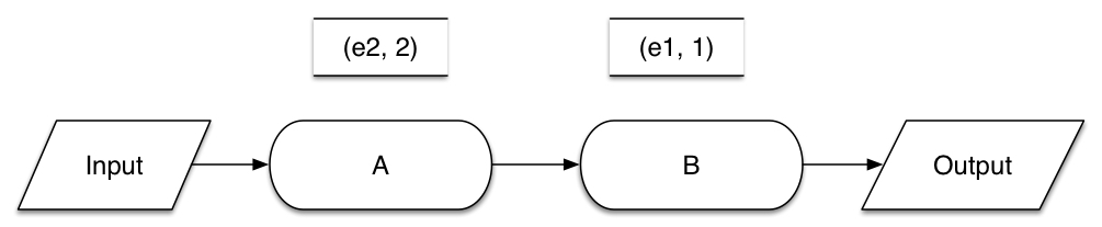
In this example, A, B are different processing vertices and each of them has one message being processed, and the OnNotify function is running on node B. For A, the number 2 in its message (e2, 2) indicates that this messages is generated in epoch 2, thus a on B counter would increase by 1 if it is counting the number of messages in epoch 1. In the example code, counts would be the counter that counts the number of distinct messages received (i.e. in other functions). Once B gets notified that one epoch has ended, the OnNotify function would be triggered, and a count for each distinct input record would then be sent to output.

Naiad can also execute cyclic dataflow programs. If there is a loop in the data flow graph, for example where the message need to be processed with the processed result of previous message, then each message circulating in the group has another counter associated with it along with the epoch. This loop counter would increase by one whenever it complete a loop once. Thus the epoch and counter can work together for the system to track progress of the whole computation.

Tracking process is not a trivial task since there are many messages with different timestamps being sent between nodes. For example, a node n is in charge of notifying the end of each epoch and performing a task ‘count the number of the event in each epoch’. Then the next question is when can n say for sure that a certain epoch has already ended thus the counting job can start. The problematic issue here is that even the node has been receiving messages with epoch e, there might still be messages with epoch e-1 that are still circulating (i.e. haven’t been consumed) in the dataflow thus if n fires the counting right now, it would end up with wrong results since those circulating messages are not counted. Naiad accomplishes this task by tracking all the messages that being sent and haven’t being successfully consumed yet, the system can then compute a could-result-in map with those messages. In a could-result-in map, a message could lead to a notification of the end of epoch e if and only if the messages has timestamp t <= e, and there is a path from the message to the notification location n and all the ingress, egress, feedback vertex on that path satisfies t <= e. This is guaranteed by that messages are not sent “back in time”. Thus the could-result-in map can keep track of the epochs, and functions rely on epochs can work correctly.

Naiad is the implementation of timely dataflow in a cluster, where the tracker on each machine would broadcast both the messages that has not been consumed and recently been consumed in order for every tracker to maintain a single view of the global could-result-in map, thus the process of the whole computation is guaranteed. Naiad also optimizes its performance by dealing with micro-stragglers such as making changes on TCP layer to reduce network latency and customizing garbage collection methods.

Another interesting point about Naiad is how it deals with failures. As described before, there are systems that achieve fault-tolerance by replication and systems such as Storm that would replay the tuple from beginning. Then we have Spark streaming, which would keep the lineage of all operations and is able to rebuilt the RDDs in parallel. Naiad more or less can be seen as an example that takes the replay approach, it would checkpoint the computation and can perform potentially more compact checkpointing when requested. When the system periodically checkpoints, all processes would pause and finish ongoing works. Then the system would perform checkpointing on each vertex and then resume. To recover from a failure, all live processes would revert to the last durable checkpoint, and the work from the failed vertex would be reassigned to other processes. This method might have higher latency for recovery due to both checkpointing and resuming than other approaches.

In short, Naiad allows processing of messages from different epochs and aggregating result from the same epoch by using timestamps on messages. Moreover, by allowing producers to set epoch on messages arbitrarily (i.e. set logical time), Naiad provides a powerful way to create batches of streams. However, the computation model of Naiad introduce high latency when dealing with failures.

Google Dataflow

We now have seen three different systems that can process data stream in large scale, however, each of them are constraint in the way of viewing the dataset. Storm can perform stream processing on each tuple, where Spark streaming and Naiad have their own way of grouping tuples together into small batches before processing. The authors of Google Dataflow (Akidau et al., 2015) believe that the fundamental problem of those views is they are limited by the processing engine, for example, if you were to use Spark streaming to process the stream, you can only group the tuples into small time intervals. The motivation of Google Dataflow is then a general underlying system with which the users can express what processing model they want.

Google Dataflow is a system that allows batch, micro-batch and stream processing where users can choose based on the tradeoffs provided by each processing model: latency or resouce constraint. Google Dataflow implements many features in order to achieve its goal, and we will briefly talk about them.

Google Dataflow provides a windowing model that supports unaligned event-time windows, which helped the users to express how to batch the tuples together in a stream. Windowing slices a dataset into finite chunks for processing as a group, one can think of it as batching as we discussed before. Unaligned windows are the windows that would only be applied to certain tuples during the period, for example, if we have an unaligned window w[1:00, 2:00)(k), and only the events with key k during the time period [1:00, 2:00) would be grouped by this window. This is powerful since it provides an alternative way of batching tuples other than just time before processing.

The next question is then how does Google Dataflow knows when to emit the results of a certain window, this requires some other signal to show when the window is done. Google Dataflow handles this by providing different choices of triggering methods. One example would be completion estimation, this is useful when combined with percentile watermarks, one might only care about processing a minimum percentage of the input data quickly than finishing every last piece of it. Another interesting triggering method is responding to data arrival, this is useful for application that are grouping data based on the number of them, for example, the processor can be fired once 100 data points are received. These real triggering semantics help Google Dataflow to become a general purposed processing system, the first method allows the users to deal with stragglers while the second one provides a way to support tuple-based windows.

In addition to controlling when results can be emitted, the system also provides a way to control how windows can relate to each other. The results can be discarding, where the contents would be discarded once triggering, this makes data storage more efficient since once the results are consumed, we can clear them from the buffers. The results can also be accumulating, once triggering, the contents are left intact and stored in persistent state, later results can become a refinement of previous results, this mode is useful when the downstream consumers are expected to overwrite old result once the new one comes, for example, we might want to write the count of a view of certain movie from the stream pipeline with low latency, and we can refine the count at the end of the day by running a slower batch process on the aggregated data. The last mode is accumulating & retracting, where in addition to accumulating semantics, a copy of the emitted value is also stored in persistent state. When the window triggers again in the future, a retraction for the previous value will be emitted first, followed by the new value, this is useful when both the results from the previous processing and the later one are needed to be combined. For example, one process is counting the number of views during a certain period, a user went offline during the window and came back after the window ended when the result of the counting c was already emitted, the process now need to retract the previous result c and indicate that the correct number should be c+1.

PCollection<KV<String, Integer>> output = input
	.apply(Window.trigger(Repeat(AtPeriod(1, MINUTE)))
		.accumulating())
	.apply(Sum.integersPerKey());

The above example code shows how to apply a trigger that repeatedly fires on one-minute period, where PCollection can be viewed as the data stream abstraction in Google Dataflow. The accumulating mode is also specified so that the Sum can be refined overtime.

Google Dataflow also relies on MillWheel (Akidau et al., 2013) as the underlying execution engine to achieve exactly-once-delivery of the tuples. MillWheel is a framework for building low-latency data-processing applications used at Google. It achieves exactly-once-delivery by first checking the incoming record and discard duplicated ones, then pending the productions (i.e., produce records to any stream) until the senders are acknowledges, only then the pending productions are sent.

In conclusion, one of the most important core principles that drives Google Dataflow is to accommodate the diversity of known use cases, it did so by providing a rich set of abstractions such as windowing, triggering and controlling. Compared to the ‘specialized’ system that we discussed above, Google Dataflow is a more general system that can fulfill batch, micro-batch, and stream processing requirements.

The systems being used nowadays

Until now we have talked about what is stream processing and what are the different model/system built for this purpose. As shown before, the systems vary on how they view stream, for example Storm can perform operation on the level of each tuple while Spark streaming could group tuples into micro-batches and then process on the level of batch. They also differ on how to deal with failures, Storm can replay the tuple from spout while Naiad would keep checkpointing. Then we introduced Google Dataflow, which seems like the most powerful tool so far that allows the users to express how to group and control the tuples in the stream.

Despite all the differences among them, they all started with more or less the same goal: to be the stream processing system that would be used by companies, and we showed several examples of why companies might need such system. In this section, we would discuss three companies that use the stream processing system as the core of their business: Alibaba, Twitter and Spotify.

Alibaba

Alibaba is the largest e-commerce retailer in the world with an annual sales more than eBay and Amazon combined in 2015. Alibaba search is its personalized search and recommendation platform which uses Apache Flink to power critical aspects of it (“Alibaba Flinke,” n.d.).

The processing engine of Alibaba runs on 2 different pipelines: a batch pipeline and a streaming pipeline, where the first one would process all data sources while the latter process updates that occur after the batch job is finished. As we can see the second pipeline is one example of stream processing. One of the example applications for the streaming pipeline is the online machine learning recommendation system. There are special days of the year (i.e. Singles Day in China, which is very similar to Black Friday in the U.S.) where transaction volume is huge and the previously-trained model would not correctly reflect the current trends, thus Alibaba needs a streaming job to take the real-time data into account. There are many reasons that Alibaba chose Flink, for example, Flink is general enough to express both the batch pipeline and the streaming pipeline. Another reason is that the changes to the products must be reflected in the final search result thus at-least-once semantics is needed, while other products in Alibaba might need exactly-once semantics, and Flink provides both semantics.

Alibaba developed a forked version of Flink called Blink to fit some of the unique requirements at Alibaba. One important improvement here is a more robust integration with YARN (“Hadoop YARN,” n.d.), where YARN is used as the global resource manager for Flink. YARN requires a job in Flink to grab all required resources up front and can not require or release resources dynamically. As Alibaba’s search engine is currently running on over 1000 machines, a better utilization of resources is critical. Blink improves on this by letting each job have its own JobMaster to request and release resources as the job requires, which optimizes the resources usage.

Twitter

Twitter is one of the ‘go-to’ examples that people would think of when considering large scale stream processing system, since it has a huge amount of data that needed to be processed in real-time. Twitter bought the company that created Storm and used Storm as its real-time analysis tool for several years. (Toshniwal et al., 2014) However, as the data volume along with the more complex use cases increased, Twitter needed to build a new real-time stream data processing system as Storm could no longer satisfy the new requirements. We would talk about how Storm was used at Twitter and then the system that they built to replace Storm-Heron.

Storm@Twitter

Twitter requires processing complex computation on streaming data in real-time since each interaction with a user requires making a number of complex decisions, often based on data that has just been created, and they use Storm as the real-time distributed stream data processing engine. As we described before, Storm represents one of the early open-source and popular stream processing systems that is in use today, and was developed by Nathan Marz at BackType which was acquired by Twitter in 2011. After the acquisition, Storm has been improved and open-sourced by Twitter and then picked up by various other organizations.

We will first briefly introduce the structure of Storm at Twitter. Storm runs on a distributed cluster, and clients submit topologies to a master node, which is in charge of distributing and coordinating the execution of the topologies. The actual bolts and spouts are tasks, and multiple tasks are grouped into executor, multiple executors are in turn grouped into a worker. The worker process would then be distributed to an actual worker node (i.e. machine), where there can be multiple worker processes be running on. Each worker node runs a supervisor that communicates with the master node thus the state of the computation can be tracked.

As shown before, Storm can guarantee each tuple is processed ‘at least once’, however, at Twitter, Storm can provide two types of semantic guarantees-“at least once” and “at most once”. “At least once” semantic is guaranteed by the directed acyclic graph as we showed before, and “at most once” semantic is guaranteed by dropping the tuple in case of a failure (e.g. by disabling the acknowledgements of each tuple). Note that for “at least once” semantic, the coordinators (i.e. Zookeeper) would checkpoint each processed tuple in the topology, and the system can start processing tuples from the last “checkpoint” that is recorded once recovered from a failure.

Storm fulfilled many requirements at Twitter with satisfactory performance. Storm was running on hundreds of servers and several hundreds of topologies ran on these clusters some of which run on more than a few hundred nodes, terabytes of data flowed through the cluster everyday and generated billions of output tuples. These topologies were used to do both simple tasks such as filtering and aggregating the content of various streams and complex tasks such as machine learning on stream data. Storm was resilient to failures and achieved relatively low latency, a machine can be taken down for maintenance without interrupting the topology and the 99% response time for processing a tuple is close to 1ms.

In conclusion, Storm was a critical infrastructure at Twitter that powered many of the real-time data-driven decisions that were made at Twitter.

Twitter Heron

Storm has long served as the core of Twitter for real-time analysis, however, as the scale of data being processed has increased, along with the increase in the diversity and the number of use cases, many limitations of Storm became apparent. (Kulkarni et al., 2015)

There are several issues with Storm that make using is at Twitter become challenging. The first challenge is debug-bility, there is no clean mapping from the logical units of computation in the topology to each physical process, this makes finding the root cause of misbehavior extremely hard. Another challenge is as the cluster resources becomes precious, the need for dedicated cluster resources in Storm leads to inefficiency and it is better to share resources across different types of systems. In addition, Twitter needs a more efficient system, simply with the increase scale, any improvement in performance can translate to huge benefit.

Twitter realized in order to meet all the needs, they needed a new real-time stream data processing system-Heron, which is API-compatible with Storm and provides significant performance improvements, lower resource consumption along with better debug-ability scalability and manageability.

A key design goal for Heron is compatibility with the Storm API, thus Heron runs topologies, graphs with spouts and bolts like Storm. Unlike Storm though, the Heron topology is translated into a physical plan before actual execution, and there are multiple components in the physical plan.

Each topology is run as an Aurora (“Apache Aurora,” n.d.) job, instead of using Nimbus (“Nimbus Project,” n.d.) as scheduler. Nimbus used to be the master node of Storm that schedules and manages all running topologies, it delopys topology on Storm, and assigns workers to execute the topology where Aurora is also a service scheduler that can manage long-running services. Twitter chose Aurora since it is developed and used by other Twitter projects. Each Aurora job is then consisted of several containers, the first container runs Topology Master, which provides a single point of contact for discovering the status of the topology and also serves as the gateway for the topology metrics through an endpoint. The other containers each run a Stream Manager, a Metrics Manager and a number of Heron Instances. The key functionality for each Stream Manager is to manage the routing of tuples efficiently, all Stream Managers are connected to each other and the tuples from Heron Instances in different containers would be transmitted through their Stream Managers, thus the Stream Managers can be viewed as Super Node for communication. Stream Manager also provides a backpressure mechanism, if the receiver component is unable to handle incoming data/tuples, then the sender can dynamically adjust the rate of the data flows through the network. For example, if the Stream Managers of the bolts are overwhelmed, they would then notice the Stream Managers of the spouts to slow down thus ensure all the data are properly processed. Heron Instance carries out the real work for a spout or a bolt, unlike worker in Storm, each Heron Instance runs only a single task as a process, in addition to performing the work, Heron Instance is also responsible for collecting multiple metrics. The metrics collected by Heron Instances would then be sent to the Metrics Manager in the same container and to the central monitoring system.

The components in the Heron topology are clearly separated, so the failure in various level would be handled differently. For example, if the Topology Master dies, the container would restart the process, and the stand-by Topology Master would take over the master while the restarted would become the stand-by. When a Stream Manager dies, it gets started in the same container, and after rediscovers the Topology Master, it would fetch and check whether there are any changes need to be made in its state. Similarly, all the other failures can be handled gracefully by Heron.

Heron addresses the challenges of Storm. First, each task is performed by a single Heron Instance, and the different functionalities are abstracted into different level, which makes debugging clearer. Second, the provisioning of resources is abstracted out thus made sharing infrastructure with other systems easier. Third, Heron provides multiple metrics along with the backpressure mechanism, which can be used to precisely reason about and achieve a consistent rate of delivering results.

Storm has been decommissioned and Heron is now the de-facto streaming system at Twitter and an interesting note is that after migrating all the topologies to Heron, there was an overall 3X reduction in hardware. Not only did Heron reduce the infrastructure needed, it also outperformed Storm by delivering 6-14X improvements in throughput, and 5-10X reductions in tuple latencies.

Spotify

Another company that deploys large scale distributed system is Spotify (“Spotify Labs,” n.d.). Every small piece of information, such as listening to a song or searching an artist, is sent to Spotify servers and processed. There are many features of Spotify that need such stream processing system, such as music/playlist recommendations. Originally, Spotify would collect all the data generated from client softwares and store them in their HDFS, and those data would then be processed on hourly basis by a batch job (i.e., the data collected each hour would be stored and processed together).

In the original Spotify structure, each job must determine, with high probability, that all data from the hourly bucket was successfully written to persistent storage before firing the job. Each job was running as a batch job by reading the files from the storage, so late-arriving data for already completed bucket could not be appended since jobs generally only read data once from a hourly bucket, thus each job has to treat late data differently. All late data is written to a currently open hourly bucket then.

Spotify then decided to use Google Dataflow, since the features provided by it is exactly what Spotify wants. The previous batch jobs can be written as streaming jobs with one hour window size, and all the data stream can be grouped based on both window and key, while the late arriving data can be gracefully handled if the controlling is set to accumulating & retracting. Also, Google Dataflow reduces the export latency of the hourly analysis results, since when assigning windows, Spotify would have an early trigger that is set to emit a pane (i.e. result) every N tuples until the window is closed.

The worst end-to-end latency observed with new Spotify system based on Google Dataflow is four times lower than the previous system and also with much lower operational overhead.

References

1. Chandrasekaran, S., Cooper, O., Deshpande, A., Franklin, M. J., Hellerstein, J. M., Hong, W., … Shah, M. A. (2003). TelegraphCQ: continuous dataflow processing. In Proceedings of the 2003 ACM SIGMOD international conference on Management of data (pp. 668–668). ACM.
2. Zaharia, M., Chowdhury, M., Das, T., Dave, A., Ma, J., McCauley, M., … Stoica, I. (2012). Resilient distributed datasets: A fault-tolerant abstraction for in-memory cluster computing. In Proceedings of the 9th USENIX conference on Networked Systems Design and Implementation (pp. 2–2). USENIX Association.
3. Apache Kafka. https://kafka.apache.org/.
4. Apache Storm. http://storm.apache.org/.
5. Zaharia, M., Das, T., Li, H., Shenker, S., & Stoica, I. (2012). Discretized streams: an efficient and fault-tolerant model for stream processing on large clusters. In Presented as part of the.
6. Murray, D. G., McSherry, F., Isaacs, R., Isard, M., Barham, P., & Abadi Martı́n. (2013). Naiad: a timely dataflow system. In Proceedings of the Twenty-Fourth ACM Symposium on Operating Systems Principles (pp. 439–455). ACM.
7. Akidau, T., Bradshaw, R., Chambers, C., Chernyak, S., Fernández-Moctezuma, R. J., Lax, R., … others. (2015). The dataflow model: a practical approach to balancing correctness, latency, and cost in massive-scale, unbounded, out-of-order data processing. Proceedings of the VLDB Endowment, 8(12), 1792–1803.
8. Toshniwal, A., Taneja, S., Shukla, A., Ramasamy, K., Patel, J. M., Kulkarni, S., … others. (2014). Storm@ twitter. In Proceedings of the 2014 ACM SIGMOD international conference on Management of data (pp. 147–156). ACM.
9. Kulkarni, S., Bhagat, N., Fu, M., Kedigehalli, V., Kellogg, C., Mittal, S., … Taneja, S. (2015). Twitter heron: Stream processing at scale. In Proceedings of the 2015 ACM SIGMOD International Conference on Management of Data (pp. 239–250). ACM.
10. Spotify Labs. https://labs.spotify.com/2016/02/25/spotifys-event-delivery-the-road-to-the-cloud-part-i/.
11. Akidau, T., Balikov, A., Bekiroğlu, K., Chernyak, S., Haberman, J., Lax, R., … Whittle, S. (2013). MillWheel: fault-tolerant stream processing at internet scale. Proceedings of the VLDB Endowment, 6(11), 1033–1044.
12. Apache Aurora. http://aurora.apache.org.
13. Nimbus Project. http://www.nimbusproject.org/docs/2.10.1/.
14. Alon, N., Matias, Y., & Szegedy, M. (1996). The space complexity of approximating the frequency moments. In Proceedings of the twenty-eighth annual ACM symposium on Theory of computing (pp. 20–29). ACM.
15. PipelineDB. https://www.pipelinedb.com/.
16. Apache Samza. http://samza.apache.org.
17. Apache Flink. https://flink.apache.org.
18. Structured Streaming. http://spark.apache.org/docs/latest/structured-streaming-programming-guide.html#overview.
19. Alibaba Flinke. http://data-artisans.com/blink-flink-alibaba-search/#more-1698.
20. Hadoop YARN. https://hadoop.apache.org/docs/r2.7.2/hadoop-yarn/hadoop-yarn-site/YARN.html.